A series of tricks and techniques I learned doing tiny GLSL demos

In the past two months or so, I spent some time making tiny GLSL demos. I wrote an article about the first one, Red Alp. There, I went into details about the whole process, so I recommend to check it out first if you're not familiar with the field.

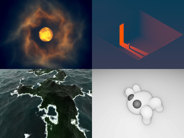
We will look at 4 demos: Moonlight, Entrance 3, Archipelago, and Cutie. But this time, for each demo, we're going to cover one or two things I learned from it. It won't be a deep dive into every aspect because it would be extremely redundant. Instead, I'll take you along a journey of learning experiences.

Moonlight

// Moonlight [460] by bµg
// License: CC BY-NC-SA 4.0
void main(){vec3 o,p,u=vec3((P+P-R)/R.y,1),Q;Q++;for(float d,a,m,i,t;i++<1e2;p=t<7.2?Q:vec3(2,1,0),d=abs(d)*.15+.1,o+=p/m+(t>9.?d=9.,Q:p/d),t+=min(m,d))for(p=normalize(u)*t,p.z-=5e1,m=max(length(p)-1e1,.01),p.z+=T,d=5.-length(p.xy*=mat2(cos(t*.2+vec4(0,33,11,0)))),a=.01;a<1.;a+=a)p.xz*=mat2(8,6,-6,8)*.1,d-=abs(dot(sin(p/a*.6-T*.3),p-p+a)),m+=abs(dot(sin(p/a/5.),p-p+a/5.));o/=4e2;O=vec4(tanh(mix(vec3(-35,-15,8),vec3(118,95,60),o-o*length(u.xy*.5))*.01),1);}

In Red Alp, I used volumetric raymarching to go through the clouds and fog, and it took quite a significant part of the code to make the absorption and emission convincing. But there is an alternative technique that is surprisingly simpler.

In the raymarching loop, the color contribution at each iteration becomes 1/d or c/d where d is the density of the material at the current ray position, and c an optional color tint if you don't want to work in grayscale level. Some variants exist, for example 1/d^2, but we'll focus on 1/d.

1/d explanation

Let's see how it looks in practice with a simple cube raymarch where we use this peculiar contribution:

void main() {
    float d, t;
    vec3 o, p,
         u = normalize(vec3(P+P-R,R.y)); // screen to world coordinate

    for (int i = 0; i < 30; i++) {
        p = u * t; // ray position

        p.z -= 3.; // take a step back

        // Rodriguez rotation with an arbitrary angle of π/2
        // and unaligned axis
        vec3 a = normalize(cos(T+vec3(0,2,4)));
        p = a*dot(a,p)-cross(a,p);

        // Signed distance function of a cube of size 1
        p = abs(p)-1.;
        d = length(max(p,0.)) + min(max(p.x,max(p.y,p.z)),0.);

        // Maxed out to not enter the solid
        d = max(d,.001);

        t += d; // stepping forward by that distance

        // Our mysterious contribution to the output
        o += 1./d;
    }

    // Arbitrary scale within visible range
    O = vec4(o/200., 1);
}

The first time I saw it, I wondered whether it was a creative take, or if it was backed by physical properties.

Let's simplify the problem with the following figure:

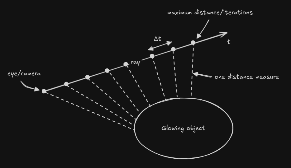
The glowing object sends photons that spread all around it. The further we go from the object, the more spread these photons are, basically following the inverse square law 1/r^2, which gives the photons density, where r is the distance to the target object.

Let's say we send a ray and want to know how many photons are present along the whole path. We have to "sum", or rather integrate, all these photons density measures along the ray. Since we are doing a discrete sampling (the dots on the figure), we need to interpolate the photons density between each sampling point as well.

Given two arbitrary sampling points and their corresponding distance d_n and d_{n+1}, any intermediate distance can be linearly interpolated with r=\mathrm{mix}(d_n,d_{n+1},t) where t is within [0,1]. Applying the inverse square law from before (1/r^2), the integrated photons density between these 2 points can be expressed with this formula (in t range):

t being normalized, the \Delta t is here to covers the actual segment distance. With the help of Sympy we can do the integration:

>>> a, b, D, t = symbols('a b D t', real=True)
>>> mix = a*(1-t) + b*t
>>> D * integrate(1/mix**2, (t,0,1)).simplify()
 D
───
a⋅b

So the result of this integration is:

Now the key is that in the loop, \Delta t stepping is actually d_{n+1}, so we end up with:

And we find back our mysterious 1/d. It's "physically correct", assuming vacuum space. Of course, reality is more complex, and we don't even need to stick to that formula, but it was nice figuring out that this simple fraction is a fairly good model of reality.

Going through the object

In the cube example we didn't go through the object, using max(d, .001). But if we were to add some transparency, we could have used d = A*abs(d)+B instead, where A could be interpreted as absorption and B the pass-through, or transparency.

I first saw this formula mentioned in Xor article on volumetric. To understand it a bit better, here is my intuitive take: the +B causes a potential penetration into the solid at the next iteration, which wouldn't happen otherwise (or only very marginally). When inside the solid, the abs(d) causes the ray to continue further (by the amount of the distance to the closest edge). Then the multiplication by A makes sure we don't penetrate too fast into it; it's the absorption, or "damping".

This is basically the technique I used in Moonlight to avoid the complex absorption/emission code.

Entrance 3

// Entrance 3 [465] by bµg
// License: CC BY-NC-SA 4.0
#define V for(s++;d<l&&s>.001;q=abs(p+=v*s)-45.,b=abs(p+vec3(mod(T*5.,80.)-7.,45.+sin(T*10.)*.2,12))-vec3(1,7,1),d+=s=min(max(p.y,-min(max(abs(p.y+28.)-17.,abs(p.z+12.)-4.),max(q.x,max(q.y,q.z)))),max(b.x,max(b.y,b.z))))
void main(){float d,s,r=1.7,l=2e2;vec3 b,v=b-.58,q,p=mat3(r,0,-r,-1,2,-1,b+1.4)*vec3((P+P-R)/R.y*20.4,30);V;r=exp(-d*d/1e4)*.2;l=length(v=-vec3(90,30,10)-p);v/=l;d=1.;V;r+=50.*d/l/l;O=vec4(pow(mix(vec3(0,4,9),vec3(80,7,2),r*r)*.01,p-p+.45),1);}

This demo was probably one of the most challenging, but I'm pretty happy with its atmospheric vibe. It's kind of different than the usual demos for this size.

I initially tried with some voxels, but I couldn't make it work with the light under 512 characters (the initialization code was too large, not the branchless DDA stepping). It also had annoying limitations (typically the animation was unit bound), so I fell back to a classic raymarching.

The first thing I did differently was to use an L-∞ norm instead of an euclidean norm for the distance function: every solid is a cube so it's appropriate to use simpler formulas.

For the light, it's not an illusion, it's an actual light: after the first raymarch to a solid, the ray direction is reoriented toward the light and the march runs again (it's the V macro). Hitting a solid or not defines if the fragment should be lighten up or not.

Mobile bugs

A bad surprise of this demo was uncovering two driver bugs on mobile:

• One with tricky for-loop compounds on Snapdragon/Adreno because I was trying hard to avoid the macros and functions.
• One with chained assignments on Imagination/PowerVR (typically affect Google Pixel Pro 10).

The first was worked around with the V macro (actually saved 3 characters in the process), but the 2nd one had to be unpacked and made me lose 2 characters.

Isometry

Another thing I studied was how to set up the camera in a non-perspective isometric or dimetric view. I couldn't make sense of the maths from the Wikipedia page (it just didn't work), but Sympy rescued me again:

# Counter-clockwise rotation
a, ax0, ax1, ax2 = symbols('a ax0:3')
c, s = cos(a), sin(a)
k = 1-c
rot = Matrix(3,3, [
    # col 1            col 2              # col 3
    ax0*ax0*k + c,     ax0*ax1*k + ax2*s, ax0*ax2*k - ax1*s, # row 1
    ax1*ax0*k - ax2*s, ax1*ax1*k + c,     ax1*ax2*k + ax0*s, # row 2
    ax2*ax0*k + ax1*s, ax2*ax1*k - ax0*s, ax2*ax2*k + c      # row 3
])

# Rotation by 45° on the y-axis
m45 = rot.subs({a:rad(-45), ax0:0, ax1:1, ax2:0})

# Apply the 2nd rotation on the x-axis to get the transform matrices for two
# classic projections
# Note: asin(tan(rad(30))) is the same as atan(sin(rad(45)))
isometric = m45 * rot.subs({a:asin(tan(rad(30))), ax0:1, ax1:0, ax2:0})
dimetric  = m45 * rot.subs({a:         rad(30),   ax0:1, ax1:0, ax2:0})

Inspecting the matrices and factoring out the common terms, we obtain the following transform matrices:

The ray direction is common to all fragments, so we use the central UV coordinate (0,0) as reference point. We push it forward for convenience: (0,0,1), and transform it with our matrix. This gives the central screen coordinate in world space. Since the obtained point coordinate is relative to the world origin, to go from that point to the origin, we just have to flip its sign. The ray direction formula is then:

To get the ray origin of every other pixel, the remaining question is: what is the smallest distance we need to step back the screen coordinates such that, when applying the transformation, the view wouldn't clip into the ground at y=0.

This requirement can be modeled with the following expression:

The -1 being the lowest y-screen coordinate (which we don't want into the ground). The lazy bum in me just asks Sympy to solve it for me:

x, z = symbols("x z", real=True)
u = m * Matrix([x, -1, z])
uz = solve(u[1] > 0, z)

We get z>\sqrt{2} for isometric, and z>\sqrt{3} for dimetric.

With an arbitrary scale S of the coordinate we end up with the following:

const float S = 50.;
vec2 u = (P+P-R)/R.y * S; // scaled screen coordinates

float A=sqrt(2.), B=sqrt(3.);

// Isometric
vec3 rd = -vec3(1)/B,
     ro = mat3(B,0,-B,-1,2,-1,A,A,A)/A/B * vec3(u, A*S + eps);

// Dimetric
vec3 rd = -vec3(B,A,B)/A/2.,
     ro = mat3(2,0,-2,-1,A*B,-1,B,A,B)/A/2. * vec3(u, B*S + eps);

The eps is an arbitrary small value to make sure the y-coordinate ends up above 0.

In Entrance 3, I used a rough approximation of the isometric setup.

Archipelago

// Archipelago [472] by bµg
// License: CC BY-NC-SA 4.0
#define r(a)*=mat2(cos(a+vec4(0,11,33,0))),
void main(){vec3 p,q,k;for(float w,x,a,b,i,t,h,e=.1,d=e,z=.001;i++<50.&&d>z;h+=k.y,w=h-d,t+=d=min(d,h)*.8,O=vec4((w>z?k.zxx*e:k.zyz/20.)+i/1e2+max(1.-abs(w/e),z),1))for(p=normalize(vec3(P+P-R,R.y))*t,p.zy r(1.)p.z+=T+T,p.x+=sin(w=T*.4)*2.,p.xy r(cos(w)*e)d=p.y+=4.,h=d-2.3+abs(p.x*.2),q=p,k-=k,a=e,b=.8;a>z;a*=.8,b*=.5)q.xz r(.6)p.xz r(.6)k.y+=abs(dot(sin(q.xz*.4/b),R-R+b)),k.x+=w=a*exp(sin(x=p.x/a*e+T+T)),p.x-=w*cos(x),d-=w;}

For this infinite procedurally generated Japan, I wanted to mark a rupture with my red/orange obsession. Technically speaking, it's actually fairly basic if you're familiar with Red Alp. I used the same noise for the mountains/islands, but the water uses a different noise.

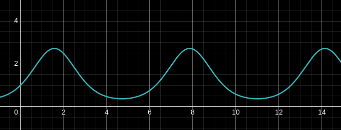
The per octave noise curve is w=exp(sin(x)), with the particularity of shifting the x coordinate with its derivative: x-=w*cos(x). This is some form of domain warping that gives the nice effect here. When I say x, I'm really referring to the x-axis position. It is not needed to work with the z-component (xz forms the flat plane) because each octave of the fbm has a rotation that "mixes" both axis, so z is actually backed in x.

Cutie

// Cutie [602] by bµg
// License: CC BY-NC-SA 4.0
#define V vec3
#define L length(p
#define C(A,B,X,Y)d=min(d,-.2*log2(exp2(X-L-A)/.2)+exp2(Y-L-B)/.2)))
#define H(Z)S,k=fract(T*1.5+s),a=V(1.3,.2,Z),b=V(1,.3*max(1.-abs(3.*k-1.),z),Z*.75+3.*max(-k*S,k-1.)),q=b*S,q+=a+sqrt(1.-dot(q,q))*normalize(V(-b.y,b.x,0)),C(a,q,3.5,2.5),C(q,a-b,2.5,2.)
void main(){float i,t,k,z,s,S=.5,d=S;for(V p,q,a,b;i++<5e1&&d>.001;t+=d=min(d,s=L+V(S-2.*p.x,-1,S))-S))p=normalize(V(P+P-R,R.y))*t,p.z-=5.,p.zy*=mat2(cos(vec4(1,12,34,1))),p.xz*=mat2(cos(sin(T)+vec4(0,11,33,0))),d=1.+p.y,C(z,V(z,z,1.2),7.5,6.),s=p.x<z?p.x=-p.x,z:H(z),s+=H(1.);O=vec4(V(exp(-i/(s>d?1e2:9.))),1);}

Here I got cocky and thought I could manage to fit it in 512 chars. I failed, by 90 characters. I did use the smoothmin operator for the first time: every limb of the body of Cutie is composed of two spheres creating a rounded cone (two sphere of different size smoothly merged like metaballs).

Then I used simple IK kinetics for the animation. Using leg parts with a size of 1 helped simplifying the formula and make it shorter.

You may be wondering about the smooth visuals itself: I didn't use the depth map but simply the number of iterations. Due to the nature of the raymarching algorithm, when a ray passes close to a shape, it slows down significantly, increasing the number of iterations. This is super useful because it exaggerate the contour of the shapes naturally. It's wrapped into an exponential, but i defines the output color directly.

What's next

I will continue making more of those, keeping my artistic ambition low because of the 512 characters constraint I'm imposing on myself.

You may be wondering why I keep this obsession about 512 characters, and many people called me out on this one. There are actually many arguments:

• A tiny demo has to focus on one or two very scoped aspects of computer graphics, which makes it perfect as a learning support.
• It's part of the artistic performance: it's not just techniques and visuals, the wizardry of the code is part of why it's so impressive. We're in an era of visuals, people have been fed with the craziest VFX ever. But have they seen them with a few hundreds bytes of code?
• The constraint helps me finish the work: when making art, there is always this question of when to stop. Here there is an intractable point where I just cannot do more and I have to move on.
• Similarly, it prevents my ambition from tricking me into some colossal project I will never finish or even start. That format has a ton of limitations, and that's its strength.
• Working on such a tiny piece of code for days/weeks just brings me joy. I do feel like a craftsperson, spending an unreasonable amount of time perfecting it, for the beauty of it.
• I'm trying to build a portfolio, and it's important for me to keep it consistent. If the size limit was different, I would have done things differently, so I can't change it now. If I had hundreds more characters, Red Alp might have had birds, the sky opening to lit a beam of light on the mountains, etc.

Why 512 in particular? It happens to be the size of a toot on my Mastodon instance so I can fit the code there, and I found it to be a good balance.