Deconstructing Bézier curves

Graphists, animators, game programmers, font designers, and other graphics professionals and enthusiasts are often working with Bézier curves. They're popular, extensively documented, and used pretty much everywhere. That being said, I find them being explained almost exclusively in 2 or 3 dimensions, which can be a source of confusion in various situations. I'll try to deconstruct them a bit further in this article. At the end or the post, we'll conclude with a concrete example where this deconstruction is helpful.

A Bézier curve in pop culture

Most people are first confronted with Bézier curves through a UI that may look like this:

In this case the curve is composed of 4 user controllable points, meaning it's a Cubic Bézier.

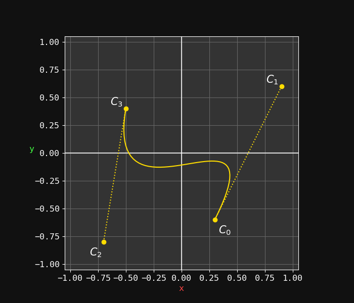
C_0, C_1, C_2 and C_3 are respectively the start, controls, and end 2D point coordinates. Evaluating this formula for all the t values within [0,1] will give all the points of the curve. Simple enough.

Now this is obvious but the important take here is that this formula applies to each dimension. Since we are working in 2D here, it is evaluated on both the x and y-axis. As a result, a more explicit writing of the formula would be:

Intuitively, you may start to see in the mathematical form how each point contributes to the curve, but it involves some tricky mental gymnastic (at least for me). So before diving into the multidimensional aspect, we will simplify the problem by looking into lower degrees.

Lower degrees

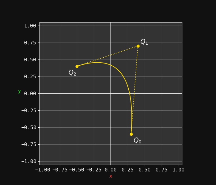
As implied by its name, the Cubic curve B_3(t) is of the 3rd degree. The 2nd most popular curve is the Quadratic curve B_2(t) where instead of 2 control points, we only have one (Q_1, in the middle):

Can we go lower? Well, there is a "1st degree Bézier curve" but you won't hear that term very often, because after removing the remaining control point:

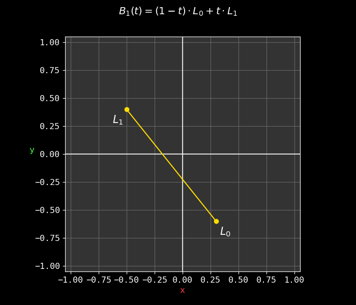
The "curve" is now a simple line between the 2 points. Still, the concept of interpolation between the points is consistent/symmetric with the cubic and the quadratic.

Do you recognize the formula (see title of the figure)? Yes, this is mix(), one of the most useful math formula! The contribution of each factor should make sense this time: t varies within [0,1], at t=0 we have 100% of L_0 (the starting point), at t=1 we have 100% of L_1, in the middle at t=\frac{1}{2} we have 50% of each, etc. All intermediate values of t define a straight line between these 2 points. We have a simple linear interpolation.

The presence of this function in the 1st degree is not just a coincidence: the \mathrm{mix} function is actually the cornerstone of all the Bézier curves. Indeed, we can build up the Bézier formulas using exclusively nested \mathrm{mix()}:

• B_1(l_0,l_1,t) = \mathrm{mix}(l_0,l_1,t)
• B_2(q_0,q_1,q_2,t) = B_1(\mathrm{mix}(q_0,q_1,t), \mathrm{mix}(q_1,q_2,t), t)
• B_3(c_0,c_1,c_2,c_3,t) = B_2(\mathrm{mix}(c_0,c_1,t), \mathrm{mix}(c_1,c_2,t), \mathrm{mix}(c_2,c_3,t))

This way of formulating the curves is basically De Casteljau's algorithm. You have no idea how much I love accidentally finding yet again a relationship with my favorite mathematical function.

But back to our "Bézier 1st degree", remember that we are still in 2D:

This multi-dimensional graphic representation can be problematic because it is exclusively spatial: if one is interested in the t parameter, it has to be extrapolated visually from a twisted curve using mind bending powers, which is not always practical.

Mono-dimensional

In order to represent t, we have to split each spatial dimension and draw them according to t (defined within [0,1]).

Let's work this out with the following cubic curve (start point is bottom-left):

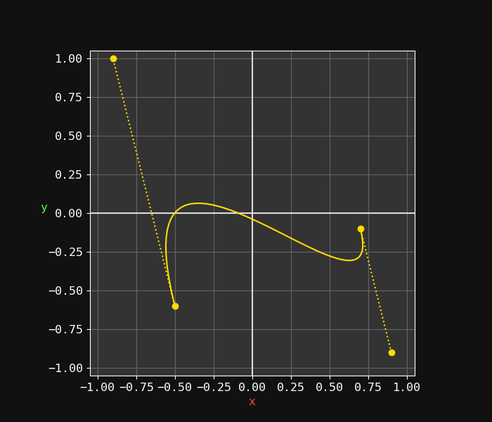
If we study this curve, we can see that the x is slightly decreasing, then increasing for most of the curve, then slightly decreasing again. In comparison, the y seems to be increasing, decreasing, then increasing again, probably more strongly than with x. But can you tell for sure what their respective curves actually look like precisely? I for sure can't, but my computer can:

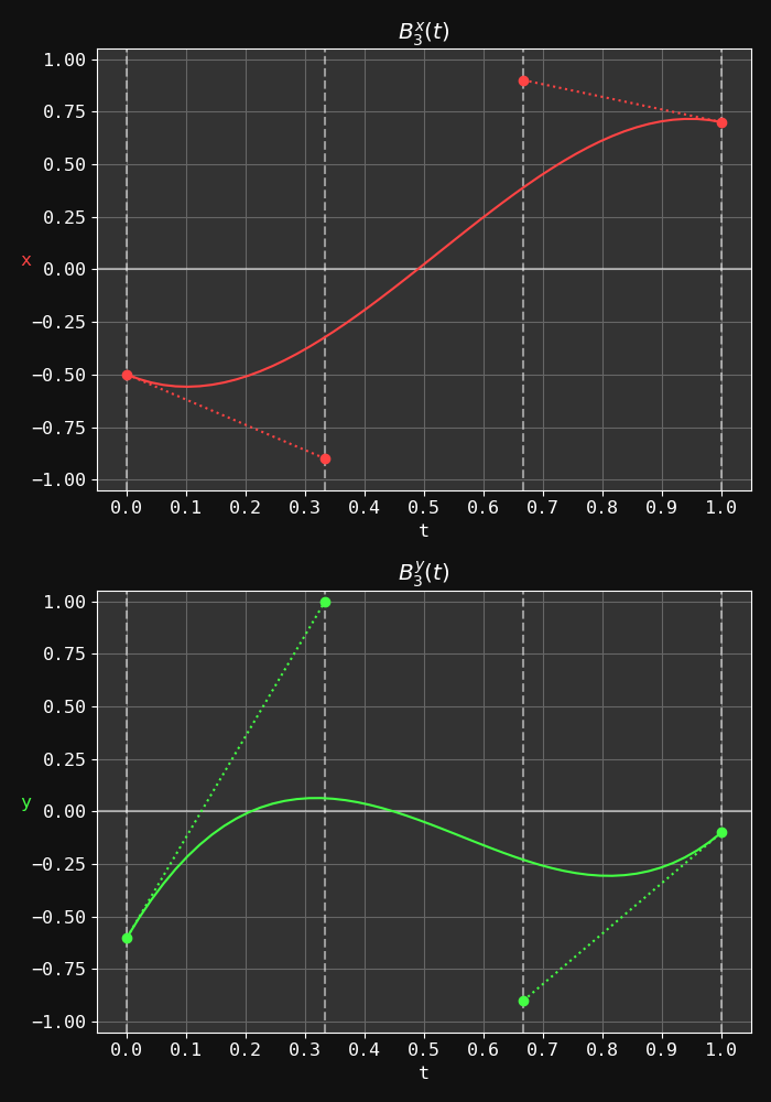
Just to be extra clear: the formula is unchanged, we're simply tracing the x and y dimensions separately according to t instead of plotting the curve in a xy plane. Note that this means C_0, C_1, C_2 and C_2 can now only change vertically: they are respectively placed at t=0, t=\frac{1}{3}, t=\frac{2}{3} and t=1. The vertical axis corresponds to their value on their respective plane.

Similarly, with a quadratic we would have Q_0 at t=0, Q_1 at t=\frac{1}{2} and Q_2 at t=1.

So what's so great about this representation? Well, first of all the curves are not going backward anymore, they can be understood by following a left-to-right reading everyone is familiar with: there is no shenanigan involved in the interpretation anymore. Also, we are now going to be able to work them out in algebraic form.

Polynomial form

So far we've looked at the curve under their Bézier form, but they can also be expressed in their polynomial form:

This algebraic form is great because we can now plug the formula into a polynomial root finding algorithm in order to identify the roots. Let's study a concrete use case of this.

Concrete use case: intersecting ray

A fundamental problem of text rendering is figuring out whether a given pixel P lands inside or outside the character shape (which is composed of a chain of Bézier curves). The most common algorithms (non-zero rule or even-odd rule) involve a ray going from the pixel position into an arbitrary direction toward infinity (usually horizontal for simplicity). If we can identify every intersection of this ray with each curve of the shape, we can deduce if our pixel point P=(P_x,P_y) is inside or outside.

We will simplify the problem to the crossing of just one curve, using the one from previous section. It would look like this with an arbitrary point P:

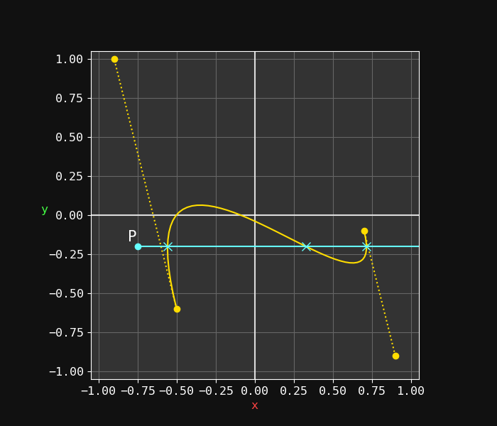
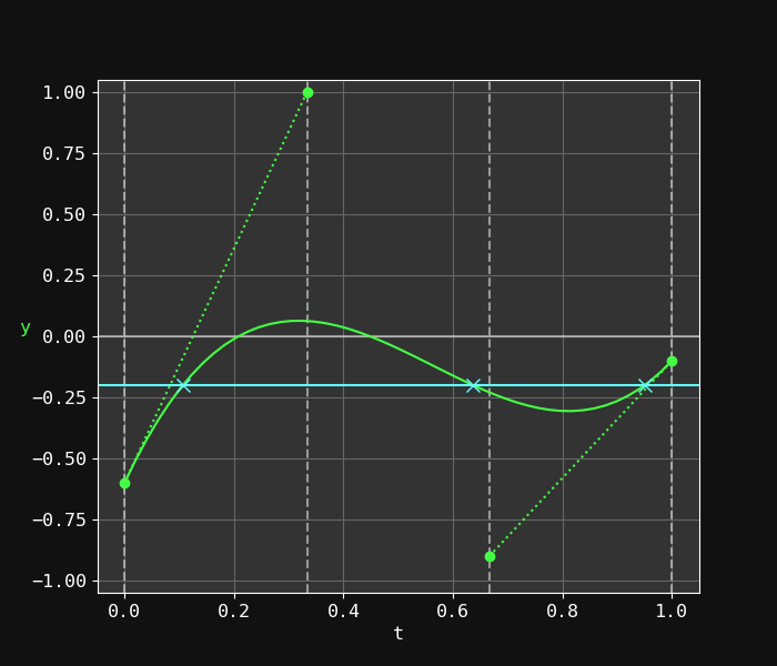
We're looking for the intersection coordinates, but how can we do that in 2D space? Well, with a horizontal ray, we would have to know when the y-coordinate of the curve is the same as the y-coordinate of P, so we first have to solve B_y(t) = P_y, or B_y(t)-P_y=0, where B_y(t) is the y component of the given Bézier curve B(t).

This is a schoolbook root finding problem, because given that B(t) is of the third degree, we end up solving the equation: a_3t^3+b_3t^2+c_3t+d_3-P_y=0 (the d₃-Py part is constant, so it acts as the last coefficient of the polynomial). This gives us the t values (or roots), that is where the ray crosses our y component.

Since this is a 3rd degree polynomial (highest power is 3), we will have at most 3 points were the ray crosses the curve. In our case, we do actually get the maximum number of roots:

Now that we have the t values on our curve (remember that t values are common for both x and y-axis), we can simply evaluate the x component of the B(t) to obtain the x coordinate.

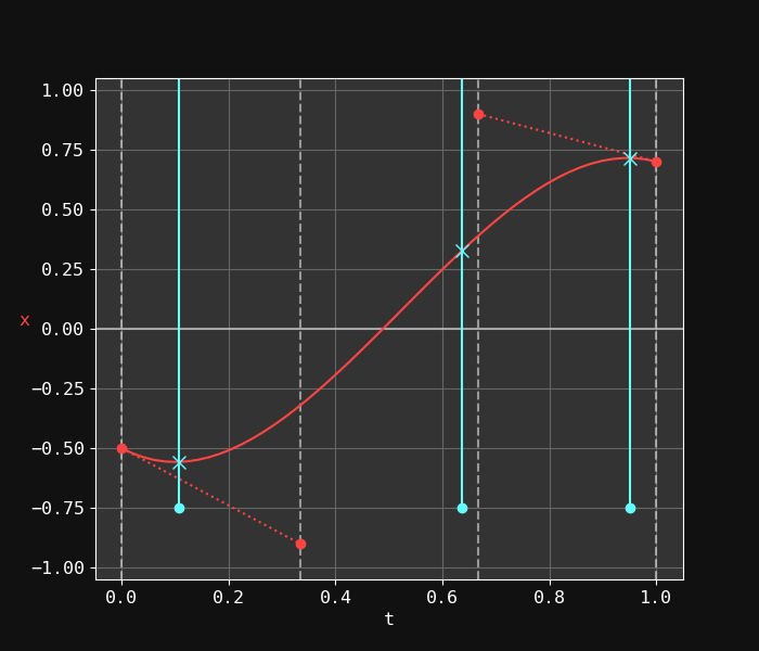
Using P_x, we can filter which roots we want to keep. In this case, P_x=-0.75, so we're going to keep all the intersections (all the roots x-coordinates are located above this value).

We could do exactly the same operation by solving B_x(t)-P_x=0 and evaluating B_y(t) on the roots we found: this would give us the intersections with a vertical ray instead of a horizontal one.

I'm voluntarily omitting a lot of technical details here, such as the root finding algorithm and floating point inaccuracies challenges: the point is to illustrate how the 1D deconstruction is essential in understanding and manipulating Bézier curves.

Bonus

During the writing of this article, I made a small matplotlib demo which got quite popular on Twitter, so I'm sharing it again:

import matplotlib.pyplot as plt
import numpy as np
from matplotlib.animation import FuncAnimation

def mix(a, b, x): return (1 - x) * a + b * x
def linear(a, b, x): return (x - a) / (b - a)
def remap(a, b, c, d, x): return mix(c, d, linear(a, b, x))

def bezier1(p0, p1, t): return mix(p0, p1, t)
def bezier2(p0, p1, p2, t): return bezier1(mix(p0, p1, t), mix(p1, p2, t), t)
def bezier3(p0, p1, p2, p3, t): return bezier2(mix(p0, p1, t), mix(p1, p2, t), mix(p2, p3, t), t)

def _main():
    pad = 0.05
    bmin, bmax = -1, 1
    x_color, y_color, xy_color = "#ff4444", "#44ff44", "#ffdd00"

    np.random.seed(0)
    r0, r1 = np.random.uniform(-1, 1, (2, 4))
    r2, r3 = np.random.uniform(0, 2 * np.pi, (2, 4))

    cfg = {
        "axes.facecolor": "333333",
        "figure.facecolor": "111111",
        "font.family": "monospace",
        "font.size": 9,
        "grid.color": "666666",
    }
    plt.style.use("dark_background")
    with plt.rc_context(cfg):
        fig = plt.figure(figsize=[8, 4.5])
        gs = fig.add_gridspec(nrows=2, ncols=3)

        ax_x = fig.add_subplot(gs[0, 0])
        ax_x.grid(True)
        for i in range(4):
            ax_x.axvline(x=i / 3, linestyle="--", alpha=0.5)
        ax_x.axhline(y=0, alpha=0.5)
        ax_x.set_xlabel("t")
        ax_x.set_ylabel("x", rotation=0, color=x_color)
        ax_x.set_xlim(0 - pad, 1 + pad)
        ax_x.set_ylim(bmin - pad, bmax + pad)
        (x_plt,) = ax_x.plot([], [], "-", color=x_color)
        (x_plt_c0,) = ax_x.plot([], [], "o:", color=x_color)
        (x_plt_c1,) = ax_x.plot([], [], "o:", color=x_color)

        ax_y = fig.add_subplot(gs[1, 0])
        ax_y.grid(True)
        for i in range(4):
            ax_y.axvline(x=i / 3, linestyle="--", alpha=0.5)
        ax_y.axhline(y=0, alpha=0.5)
        ax_y.set_xlabel("t")
        ax_y.set_ylabel("y", rotation=0, color=y_color)
        ax_y.set_xlim(0 - pad, 1 + pad)
        ax_y.set_ylim(bmin - pad, bmax + pad)
        (y_plt,) = ax_y.plot([], [], "-", color=y_color)
        (y_plt_c0,) = ax_y.plot([], [], "o:", color=y_color)
        (y_plt_c1,) = ax_y.plot([], [], "o:", color=y_color)

        ax_xy = fig.add_subplot(gs[0:2, 1:3])
        ax_xy.grid(True)
        ax_xy.axvline(x=0, alpha=0.8)
        ax_xy.axhline(y=0, alpha=0.8)
        ax_xy.set_aspect("equal", "box")
        ax_xy.set_xlabel("x", color=x_color)
        ax_xy.set_ylabel("y", rotation=0, color=y_color)
        ax_xy.set_xlim(bmin - pad, bmax + pad)
        ax_xy.set_ylim(bmin - pad, bmax + pad)
        (xy_plt,) = ax_xy.plot([], [], "-", color=xy_color)
        (xy_plt_c0,) = ax_xy.plot([], [], "o:", color=xy_color)
        (xy_plt_c1,) = ax_xy.plot([], [], "o:", color=xy_color)

        fig.tight_layout()

        def update(frame):
            px = remap(-1, 1, bmin, bmax, np.sin(r0 * frame + r2))
            py = remap(-1, 1, bmin, bmax, np.sin(r1 * frame + r3))
            t = np.linspace(0, 1)
            x = bezier3(px[0], px[1], px[2], px[3], t)
            y = bezier3(py[0], py[1], py[2], py[3], t)

            x_plt.set_data(t, x)
            x_plt_c0.set_data((0, 1 / 3), (px[0], px[1]))
            x_plt_c1.set_data((2 / 3, 1), (px[2], px[3]))

            y_plt.set_data(t, y)
            y_plt_c0.set_data((0, 1 / 3), (py[0], py[1]))
            y_plt_c1.set_data((2 / 3, 1), (py[2], py[3]))

            xy_plt.set_data(x, y)
            xy_plt_c0.set_data((px[0], px[1]), (py[0], py[1]))
            xy_plt_c1.set_data((px[2], px[3]), (py[2], py[3]))

        duration, fps, speed = 15, 60, 3
        frames = np.linspace(0, duration * speed, duration * fps)
        anim = FuncAnimation(fig, update, frames=frames)
        anim.save("/tmp/bezier.webm", fps=fps, codec="vp9", extra_args=["-preset", "veryslow", "-tune-content", "screen"])


if __name__ == "__main__":
    _main()