Fixing the iterative damping interpolation in video games

As I'm exploring the fantastic world of indie game development lately, I end up watching a large number of video tutorials on the subject. Even though the quality of the content is pretty variable, I'm very grateful to the creators for it. That being said, I couldn't help noticing this particular bit times and times again:

a = lerp(a, B, delta * RATE)

Behind this apparent banal call hides a terrible curse, forever perpetrated by innocent souls on the Internet.

In this article we will study what it's trying to achieve, how it works, why it's wrong, and then we'll come up with a good solution to the initial problem.

The usual warning: I don't have a mathematics or academic background, so the article is addressed at other neanderthals like myself, who managed to understand that pressing keys on a keyboard make pixels turn on and off.

What is it?

Let's start from the beginning. We're in a game engine main loop callback called at a regular interval (roughly), passing down the time difference from the last call.

In Godot engine, it looks like this:

func _physics_process(delta: float):
    ...

If the game is configured to refresh at 60 FPS, we can expect this function to be called around 60 times per second with delta = 1/60 = 0.01666....

As a game developer, we want some smooth animations for all kind of transformations. For example, we may want the speed of the player to go down to zero as they release the moving key. We could do that linearly, but to make the stop less brutal and robotic we want to slow down the speed progressively.

linear vs exponential GIF — Linear (top) versus smooth/exponential (bottom) animation

Virtually every tutorial will suggest updating some random variable with something like that:

velocity = lerp(velocity, 0, delta * RATE)

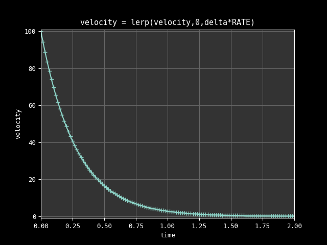
At 60 FPS, a decay RATE defined to 3.5, and an initial velocity of 100, the velocity will go down to 0 following this curve:

velocity curve — Example curve of a decaying variable

Note: velocity is just a variable name example, it can be found in many other contexts

If you're familiar with lerp() ("linear interpolation") you may be wondering why this is making a curve. Indeed, this lerp() function, also known as mix(), is a simple linear function defined as lerp(a,b,x) = x*(b-a) + a or its alternative stable form lerp(a,b,x) = (1-a)x + bx. For more information, see a previous article about this particular function. But here we are re-using the previous value, so this essentially means nesting lerp() function calls, which expands into a power formula, forming a curve composed of a chain of small straight segments.

Why is it wrong?

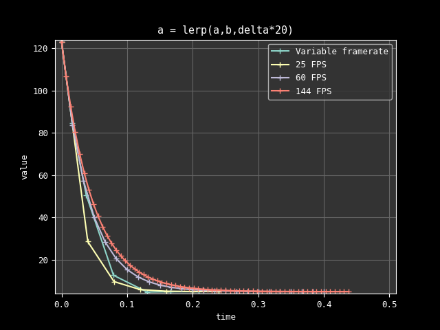
The main issue is that the formula is heavily depending on the refresh rate. If the game is supposed to work at 30, 60, or 144 FPS, then it means the physics engine is going to behave differently.

Here is an illustration of the kind of instability we can expect:

Comparison of the curves at different frame rates with the problematic formula

Note that the inaccuracy when compared to an ideal curve is not the issue here. The problem is that the game mechanics are different depending on the hardware, the system, and the wind direction observed in a small island of Japan. Imagine being able to jump further if we replace our 60Hz monitor with a 144Hz one, that would be some nasty pay to win incentive.

We may be able to get away with this by forcing a constant refresh rate for the game and consider this a non-issue (I'm not convinced this is achievable on all engines and platforms), but then we meet another problem: the device may not be able to hold this requirement at all times because of potential lags (for reasons that may be outside our control). That's right, so far we assumed delta=1/FPS but that's merely a target, it could fluctuate, causing mild to dramatic situations gameplay wise.

One last issue with that formula is the situation of a huge delay spike, causing an overshooting of the target. For example if we have RATE=3 and we end up with a frame that takes 500ms for whatever random reason, we're going to interpolate with a value of 1.5, which is way above 1. This is easily fixed by maxing out the 3rd argument of lerp to 1, but we have to keep that issue in mind.

To summarize, the formula is:

not frame rate agnostic ❌
non deterministic ❌
vulnerable to overshooting ❌

If you're not interested in the gory details on the how, you can now jump straight to the conclusion for a better alternative.

Study

We're going to switch to a more mathematical notation from now on. It's only going to be linear algebra, nothing particularly fancy, but we're going to make a mess of 1 letter symbols, bear with me.

Let's name the exhaustive list of inputs of our problem:

initial value: a_0=\Alpha (from where we start, only used once)
target value: \Beta (where we are going, constant value)
time delta: \Delta_n (time difference from last call)
the rate of change: R (arbitrary scaling user constant)
original sequence: a_{n+1} = \texttt{lerp}(a_n, \Beta, R\Delta_n) (the code in the main loop callback)
frame rate: F (the target frame rate, for example 60 FPS)
time: t (animation time elapsed)

What we are looking for is a new sequence formula u_n (u standing for purfect) that doesn't have the 3 previously mentioned pitfalls.

The first thing we can do is to transform this recursive sequence into the expected ideal contiguous time based function. The original sequence was designed for a given rate R and FPS F: this means that while \Delta_n changes in practice every frame, the ideal function we are looking for is constant: \Delta=1/F.

So instead of starting from a_{n+1} = \texttt{lerp}(a_n, \Beta, R\Delta_n), we will look for u_n starting from u_{n+1} = \texttt{lerp}(u_n, \Beta, R\Delta) with u_0=a_0=\Alpha.

Since I'm lazy and incompetent, we are just going to ask WolframAlpha for help finding the solution to the recursive sequence. But to feed its input we need to simplify the terms a bit:

\begin{split} u_{n+1} &= \texttt{lerp}(u_n, \Beta, R\Delta) \\ &= u_n(1-R\Delta) + \Beta R\Delta \\ &= u_nP + Q \end{split}

...with P=(1-R\Delta) and Q=\Beta R\Delta. We do that so we have a familiar ax+b linear form.

According to WolframAlpha this is equivalent to:

u_n = \Alpha P^n + \frac{Q(P^n-1)}{P-1}

This is great because we now have the formula according to n, our frame number. We can also express that discrete sequence into a contiguous function according to the time t:

f(t) = \Alpha P^{tF} + \frac{Q(P^{tF}-1)}{P-1}

Expanding our temporary P and Q placeholders with their values and unrolling, we get:

\begin{split} f(t) &= AP^{tF} + \frac{Q(P^{tF}-1)}{P-1} \\ &= A(1-R\Delta)^{tF} + \frac{\Beta R\Delta((1-R\Delta)^{tF}-1)}{(1-R\Delta)-1} \\ &= A(1-R\Delta)^{tF} - \Beta((1-R\Delta)^{tF}-1) \\ &= A(1-R\Delta)^{tF} + \Beta(1-(1-R\Delta)^{tF}) \\ &= \texttt{lerp}(\Beta, \Alpha, (1-R\Delta)^{tF}) \\ &= \texttt{lerp}(\Beta, \Alpha, (1-R/F)^{tF}) \\ f(t) &= \boxed{\texttt{lerp}(\Alpha, \Beta, 1-(1-R/F)^{tF})} \end{split}

This function perfectly matches the initial lerp() sequence in the hypothetical situation where the frame rate is honored. Basically, it's what the sequence a_{n+1} was meant to emulate at a given frame rate F.

Note: we swapped the first 2 terms of lerp() at the last step because it makes more sense semantically to go from \Alpha to \Beta.

Let's again summarize what we have and what we want: we're into the game main loop and we want our running value to stick to that f(t) function. We have:

v=f(t): the value previously computed (t is the running duration so far, but we don't have it); in the original sequence this is known as a_n
\Delta_n: the delta time for the current frame

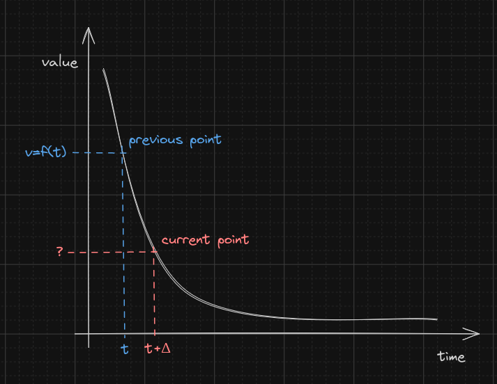
We are looking for a function \Eta(v,\Delta_n) which defines the position of a new point on the curve, only knowing v and \Delta_n. It's a "time agnostic" version of f(t).

Basically, it is defined as \Eta(v,\Delta_n)=f(t+\Delta_n), but since we don't have t it's not very helpful. That being said, while we don't have t, we do have f(t) (the previous value v).

Looking at the curve, we know the y-value of the previous point, and we know the difference between the new point and the previous point on the x-axis:

previous to current point — Previous and current point in time

If we want t (the total time elapsed at the previous point), we need the inverse function f^{-1}. Indeed, t = f^{-1}(f(t)): taking the inverse of a function gives back the input. We know f so we can inverse it, relying on WolframAlpha again (what a blessing this website is):

f^{-1}(x) = \frac{\ln{\frac{\Beta-x}{\Beta-\Alpha}}}{F \ln(1-R/F)}

Note: \ln stands for natural logarithm, sometimes also called \log. Careful though, on Desmos for example \log is in base 10, not base e (while its \exp is in base e for some reason).

This complex formula may feel a bit intimidating but we can now find \Eta only using its two parameters:

\begin{split} \Eta(v,\Delta_n) &= f(t + \Delta_n) \\ &= f(f^{-1}(f(t)) + \Delta_n) \\ &= f(f^{-1}(v) + \Delta_n) \\ &= f(\frac{\ln{\frac{\Beta-v}{\Beta-\Alpha}}}{F \ln(1-R/F)} + \Delta_n) \\ &= \texttt{lerp}(\Alpha, \Beta, 1-(1-R/F)^{(\frac{\ln{\frac{\Beta-v}{\Beta-\Alpha}}}{F \ln(1-R/F)} + \Delta_n) \times F}) \\ &= \texttt{lerp}(\Alpha, \Beta, 1-(1-R/F)^{\frac{\ln{\frac{\Beta-v}{\Beta-\Alpha}}}{\ln(1-R/F)}} (1-R/F)^{F\Delta_n}) \\ &= \texttt{lerp}(\Alpha, \Beta, 1-\frac{\Beta-v}{\Beta-\Alpha} (1-R/F)^{F\Delta_n}) \\ &= (1-\frac{\Beta-v}{\Beta-\Alpha} (1-R/F)^{F\Delta_n})(\Beta-\Alpha) + A \\ &= (\Beta-\Alpha) - (\Beta-v) (1-R/F)^{F\Delta_n} + A \\ &= (v-\Beta)(1-R/F)^{F\Delta_n} + \Beta \\ &= \texttt{lerp}(\Beta, v, (1-R/F)^{F\Delta_n}) \\ \Eta(v,\Delta_n) &= \texttt{lerp}(v, \Beta, 1-(1-R/F)^{F\Delta_n}) \end{split}

Again we swapped the first 2 arguments of lerp at the last step at the cost of an additional subtraction: this is more readable because \Beta is our destination point.

An interesting property that is going to be helpful here is m^n = e^{n \ln{m}}. For my fellow programmers getting tensed here: pow(m, n) == exp(n * log(m)). Replacing the power with the exponential may not seem like an improvement at first, but it allows packing all the constant terms together:

\begin{split} \Eta(v,\Delta_n) &= \texttt{lerp}(v, \Beta, 1-(1-R/F)^{F\Delta_n}) \\ &= \texttt{lerp}(v, \Beta, 1-e^{F\ln(1-R/F)\Delta_n}) \end{split}

F\ln(1-R/F) can be pre-computed because it is constant: it's our rate conversion formula, which we can extract:

\begin{split} R' &= F\ln(1-R/F) \\ \Eta(v,\Delta_n) &= \texttt{lerp}(v, \Beta, 1-e^{R'\Delta_n}) \end{split}

Rewriting this in a sequence notation, we get:

\begin{split} R' &= F\ln(1-R/F) \\ u_{n+1} &= \texttt{lerp}(u_n, \Beta, 1-e^{R'\Delta_n}) \end{split}

We're going to make one last adjustment: R' is negative, which is not exactly intuitive to work with as a user (in case it is defined arbitrarily and not through the conversion formula), so we make a sign swap for convenience:

\boxed{\begin{split} R' &= -F\ln(1-R/F) \\ u_{n+1} &= \texttt{lerp}(u_n, \Beta, 1-e^{-R'\Delta_n}) \end{split}}

The conversion formula is optional, it's only needed to port a previously broken code to the new formula. One interesting thing here is that R' is fairly close to R when R is small.

For example, a rate factor R=5 at 60 FPS gives us R' \approx 5.22. This means that if the rate factors weren't closely tuned, it is probably acceptable to go with R'=R and not bother with any conversion. Still, having that formula can be useful to update all the decay constants and check that everything still works as expected.

Also, notice how if the delta gets very large, -R'\Delta_n is going toward -\infty, e^{-R'\Delta_n} toward 0, 1-e^{-R'\Delta_n} toward 1, and so the interpolation is going to reach our final target \Beta without overshooting. This means the formula doesn't need any extra care with regard to the 3rd issue we pointed out earlier.

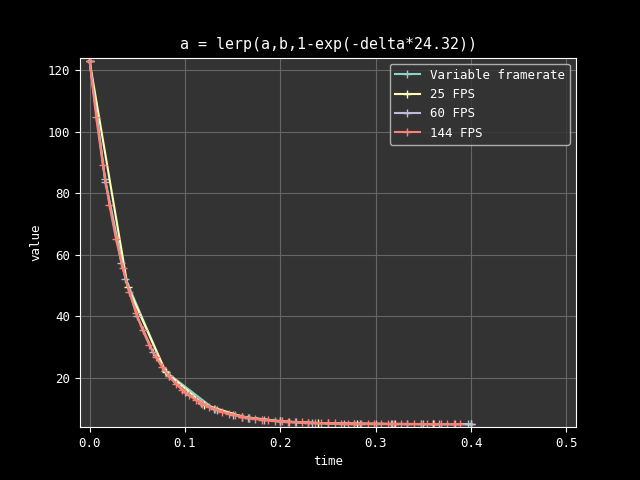
Looking at the previous curves but now with the new formula and an adjusted rate:

Conclusion

So there we have it, the perfect formula, frame rate agnostic ✅, deterministic ✅ and resilient to overshooting ✅. If you've quickly skimmed through the maths, here is what you need to know:

a = lerp(a, B, delta * RATE)

Should be changed to:

a = lerp(a, B, 1.0 - exp(-delta * RATE2))

With the precomputed RATE2 = -FPS * log(1 - RATE/FPS) (where log is the natural logarithm), or simply using RATE2 = RATE as a rough equivalent.

Also, any existing overshooting clamping can safely be dropped.

Now please adjust your game to make the world a better and safer place for everyone ♥

Going further

As suggested on HN:

for numerical stability it makes sense to use -expm1(x) instead of 1-exp(x)
API wise, proposing a time constant T instead of the rate (where T=1/rate) might be more intuitive
for performance reasons, the exponential could be expanded manually to x+x²/2 for small value of x

For updates and more frequent content you can follow me on Mastodon. Feel also free to subscribe to the RSS in order to be notified of new write-ups. It is also usually possible to reach me through other means (check the footer below). Finally, discussions on some of the articles can sometimes be found on HackerNews, Lobste.rs and Reddit.