These last years, in the context of working on a graphic rendering engine, I've been confronted to many engineering problems involving mathematics: basic geometry, colorimetry, curves, animations, video, etc. In all these situations, I needed at some point to formalize a "space conversion" of some sort.
My mathematical background is extremely fragile, but coming up with some very basic tooling for these operations helped me building up my mental models so much faster. These formulas were by far the most impactful in my daily struggle with maths.
Formula 1: from normalized input to whatever output
Anytime you try to abstract a concept mathematically, you're usually working
within the [0,1] range, the "purest" data form representation. This is often
referred as the "normalized form". When we have a value in this range, we can
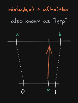
map it to any range using a mix() function, also known as lerp():

The function is known to have 2 forms, both having their use-case:
mix(a,b,x) = a*(1-x) + bxmix(a,b,x) = x*(b-a) + a
The first one is numerically stable, meaning that's the form we usually want to use in the code, because it will lead to less floating point inaccuracies.
But the 2nd one is also useful because it does not repeat the x input. I find
it handy to work with when doing substitution in basic algebra. It also notably
follows the well-known polynomial form. Finally, It's also easier to
reason with: b-a represents the total distance ("end minus start"), + a
represents the offsetting, and x represents the "amount" of the distance.
Out of all the formulas in the article, this is the most popular one. It's often referred as the "linear interpolation", but I don't like this naming because it directly conflicts with the 2nd formula doing the exact opposite.
It's so popular that GLSL does have it builtin. The wide variety of applications makes it impossible to make an exhaustive list, but if I had to pick one example it would be the mix of two colors when doing a gradient: if you want a certain percentage of a color, and the remaining of another color, this is what you will use (let's ignore gamma correction for now, alright?).
Formula 2: from whatever input to a normalized output
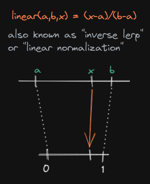
This 2nd formula is also a "linear interpolation", except it's the exact
opposite: we're going from an arbitrary range to a normalized one. The use of
the same term to refer to both functions was a huge source of confusion for me
in the past. Since this function has no official name, I will simply refer to
it as linear(a,b,x) = (x-a)/(b-a), or sometimes linear_norm(). Some people
also like to call it "inverse lerp":

This complements mix() in such an elegant way, it's a real shame it has no
"official" name. The usefulness of this function is basically to provide a way
of normalizing a value from any space/range. Said differently, this function is
a way of getting a standard and re-usable answer to the question "where is x
located between a and b?"
Formula 3: From whatever input to whatever output
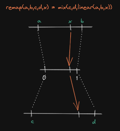
Now with the help of mix() and linear() we can now go from one range to any
other: remap(a,b,c,d,x) = mix(c,d,linear(a,b,x)).

The logic is pretty straightforward: we have a value in the range [a,b],
which we first normalize with linear(), then we directly use that result to
signify where we want to land on [c,d] using mix().
If you develop the expression, you will get the following useful polynomial
form: remap(a,b,c,d,x) = x*(d-c)/(b-a) + c-a*(d-c)/(b-a). Or simply
remap(a,b,c,d,x) = (x-a)*(d-c)/(b-a) + c.
Step and non-linear variants
You may see linearstep() in the wild, which is simply linear()
with a [0,1] clamping: linearstep(a,b,x) = saturate(linear(a,b,x)) (which
is useful in case x is outside [a,b]).
If you've worked with GLSL, you might have also heard of
smoothstep(). Instead of being linear, it follows a curve, but
in its implementation it's using linearstep() (hence the "step"), then bends
the results ("smooth") using a Hermite polynomial:
smoothstep(a,b,x) = 3t²-2t³ with t = linearstep(a,b,x)
Bonus: relationship between these formulas
If like me you're wondering why mix() and linear() look so different even
though their concept is so close, following is a demonstration for going from
one formula to another with basic algebra:
mix → linear
y = a*(1-x)+bx
y = a - ax + bx
y = a + bx - ax
y-a = x * (b-a)
x = (y-a)/(b-a)
linear → mix
x = (y-a)/(b-a)
x*(b-a) = y-a
bx - ax + a = y
y = a*(1-x)+bx
Conclusion
I'm sure many of the people reading this will sigh at such elementary maths,
but nowadays, not a week passes without me looking at the visual representation
of mix() and linear() when building various mental models for the concepts
I work with. I'm hoping this will be useful to other people.