In 2015, I wrote an article about how the palette color quantization was improved in FFmpeg in order to make nice animated GIF files. For some reason, to this day this is one of my most popular article.
As time passed, my experience with colors grew and I ended up being quite ashamed and frustrated with the state of these filters. A lot of the code was naive (when not terribly wrong), despite the apparent good results.
One of the major change I wanted to do was to evaluate the color distances using a perceptually uniform color space, instead of using a naive euclidean distance of RGB triplets.
As usual it felt like a week-end long project; after all, all I have to do is change the distance function to work in a different space, right? Well, if you're following my blog you might have noticed I've add numerous adventures that stacked up on each others:
- I had to work out the colorspace with integer arithmetic first
- ...which forced me to look into integer division more deeply
- ...which confronted me to all sort of undefined behaviours in the process
And when I finally reached the point where I could make the switch to OkLab (the perceptual colorspace), a few experiments showed that the flavor of the core algorithm I was using might contain some fundamental flaws, or at least was not implementing optimal heuristics. So here we go again, quickly enough I find myself starting a new research study in the pursuit of understanding how to put pixels on the screen. This write-up is the story of yet another self-inflicted struggle.
Palette quantization
But what is palette quantization? It essentially refers to the process of reducing the number of available colors of an image down to a smaller subset. In sRGB, an image can have up to 16.7 million colors. In practice though it's generally much less, to the surprise of no one. Still, it's not rare to have a few hundreds of thousands different colors in a single picture. Our goal is to reduce that to something like 256 colors that represent them best, and use these colors to create a new picture.
Why you may ask? There are multiple reasons, here are some:
- Improve size compression (this is a lossy operation of course, and using dithering on top might actually defeat the original purpose)
- Some codecs might not support anything else than limited palettes (GIF or subtitles codecs are examples)
- Various artistic purposes
Following is an example of a picture quantized at different levels:
| Original (26125 colors) | Quantized to 8bpp (256 colors) | Quantized to 2bpp (4 colors) |
|---|---|---|
 |
 |
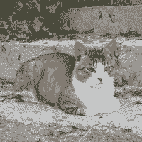 |
This color quantization process can be roughly summarized in a 4-steps based process:
- Sample the input image: we build a histogram of all the colors in the picture (basically a simple statistical analysis)
- Design a colormap: we build the palette through various means using the histograms
- Create a pixel mapping which associates a color (one that can be found in the input image) with another (one that can be found in the newly created palette)
- Image quantizing: we use the color mapping to build our new image. This step may also involve some dithering.
The study here will focus on step 2 (which itself relies on step 1).
Colormap design algorithms
A palette is simply a set of colors. It can be represented in various ways, for example here in 2D and 3D:
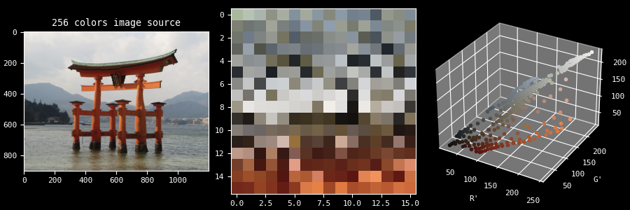
To generate such a palette, all sort of algorithms exists. They are usually classified into 2 large categories:
- Dividing/splitting algorithms (such as Median-Cut and its various flavors)
- Clustering algorithms (such as K-means, maximin distance, (E)LBG or pairwise clustering)
The former are faster but non-optimal while the latter are slower but better. The problem is NP-complete, meaning it's possible to find the optimal solution but it can be extremely costly. On the other hand, it's possible to find "local optimums" at minimal cost.
Since I'm working within FFmpeg, speed has always been a priority. This was the reason that motivated me to initially implement the Median-Cut over a more expensive algorithm.
The rough picture of the algorithm is relatively easy to grasp. Assuming we
want a palette of K colors:
- A set
Sof all the colors in the input picture is constructed, along with a respective setWof the weight of each color (how much they appear) - Since the colors are expressed as RGB triplets, they can be encapsulated in one big cuboid, or box
- The box is cut in two along one of the axis (R, G or B) on the median (hence the name of the algorithm)
- If we don't have a total
Kboxes yet, pick one of them and go back to previous step - All the colors in each of the
Kboxes are then averaged to form the color palette entries
Here is how the process looks like visually:
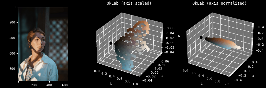
You may have spotted in this video that the colors are not expressed in RGB but in Lab: this is because instead of representing the colors in a traditional RGB colorspace, we are instead using the OkLab colorspace which has the property of being perceptually uniform. It doesn't really change the Median Cut algorithm, but it definitely has an impact on the resulting palette.
One striking limitation of this algorithm is that we are working exclusively with cuboids: the cuts are limited to an axis, we are not cutting along an arbitrary plane or a more complex shape. Think of it like working with voxels instead of more free-form geometries. The main benefit is that the algorithm is pretty simple to implement.
Now the description provided earlier conveniently avoided describing two important aspects happening in step 3 and 4:
- How do we choose the next box to split?
- How do we choose along which axis of the box we make the cut?
I pondered about that for a quite a long time.
An overview of the possible heuristics
In bulk, some of the heuristics I started thinking of:
- Should we take the box that has the longest axis across all boxes?
- Should we take the box that has the largest volume?
- Should we take the box that has the biggest Mean Squared Error when compared to its average color?
- Should we take the box that has the axis with the biggest MSE?
- Assuming we choose to go with the MSE, should it be normalized across all boxes?
- Should we even account for the weight of each color or consider them equal?
- what about the axis? Is it better to pick the longest or the one with the higher MSE?
I tried to formalize these questions mathematically to the best of my limited
abilities. So let's start by saying that all the colors c of a given box are
stored in a N×M 2D-array following the matrix notation:
| L₁ | L₂ | L₃ | … | Lₘ |
| a₁ | a₂ | a₃ | … | aₘ |
| b₁ | b₂ | b₃ | … | bₘ |
N is the number of components (3 in our case, whether it's RGB or Lab), and
M the number of colors in that box. You can visualize this as a list of
vectors as well, where c_{i,j} is the color at row i and column j.
With that in mind we can sketch the following diagram representing the tree of heuristic possibilities to implement:
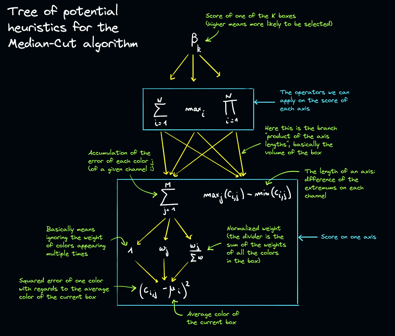
Mathematicians are going to kill me for doodling random notes all over this perfectly understandable symbols gibberish, but I believe this is required for the human beings reading this article.
In summary, we end up with a total of 24 combinations to try out:
- 2 axis selection heuristics:
- Cut the axis with the maximum error squared
- Cut the axis with the maximum length
- 3 operators:
- Maximum measurement out of all the channels
- Product of the measurements of all the channels
- Sum of the measurements of all the channels
- 4 measurements:
- Error squared, honoring weights
- Error squared, not honoring weights
- Error squared, honoring weights, normalized
- Length of the axis
If we start to intuitively think about which ones are likely going to perform the best, we quickly realize that we haven't actually formalized what we are trying to achieve. Such a rookie mistake. Clarifying this will help us getting a better feeling about the likely outcome.
I chose to target an output that minimizes the MSE against the reference image, in a perceptual way. Said differently, trying to make the perceptual distance between an input and output color pixel as minimal as possible. This is an arbitrary and debatable target, but it's relatively simple and objective to evaluate if we have faith in the selected perceptual model. Another appropriate metric could have been to find the ideal palette through another algorithm, and compare against that instead. Doing that unfortunately implied that I would trust that other algorithm, its implementation, and that I have enough computing power.
So to summarize, we want to minimize the MSE between the input and output, evaluated in the OkLab color space. This can be expressed with the following formula:
Where:
- P is a partition (which we constrain to a box in our implementation)
- C the set of colors in the partition P
- w the weight of a color
- c a single color
- \mu the average color of the set C
Special thanks to criver for helping me a ton on the math area, this last
formula is from them.
Looking at the formula, we can see how similar it is to certain branches of the heuristics tree, so we can start getting an intuition about the result of the experiment.
Experiment language
Short deviation from the main topic (feel free to skip to the next section): working in C within FFmpeg quickly became a hurdle more than anything. Aside from the lack of flexibility, the implicit casts destroying the precision deceitfully, and the undefined behaviours, all kind of C quirks went in the way several times, which made me question my sanity. This one typically severely messed me up while trying to average the colors:
#include <stdio.h>
#include <stdint.h>

int main (void)
{
    const int32_t x = -30;
    const uint32_t y = 10;

    const uint32_t a = 30;
    const int32_t b = -10;

    printf("%d×%u=%d\n", x, y, x * y);
    printf("%u×%d=%d\n", a, b, a * b);
    printf("%d/%u=%d\n", x, y, x / y);
    printf("%u/%d=%d\n", a, b, a / b);
    return 0;
}
% cc -Wall -Wextra -fsanitize=undefined test.c -o test && ./test
-30×10=-300
30×-10=-300
-30/10=429496726
30/-10=0
Anyway, I know this is obvious but if you aren't already doing that I suggest you build your experiments in another language, Python or whatever, and rewrite them in C later when you figured out your expected output.
Re-implementing what I needed in Python didn't take me long. It was, and still
is obviously much slower at runtime, but that's fine. There is a lot of room
for speed improvement, typically by relying on numpy (which I didn't bother
with).
Experiment results
I created a research repository for the occasion. The code to reproduce and the results can be found in the color quantization README.
In short, based on the results, we can conclude that:
- Overall, the box that has the axis with the largest non-normalized weighted sum of squared error is the best candidate in the box selection algorithm
- Overall, cutting the axis with the largest weighted sum of squared error is the best axis cut selection algorithm
To my surprise, normalizing the weights per box is not a good idea. I initially observed that by trial and error, which was actually one of the main motivator for this research. I initially thought normalizing each box was necessary in order to compare them against each others (such that they are compared on a common ground). My loose explanation of the phenomenon was that not normalizing causes a bias towards boxes with many colors, but that's actually exactly what we want. I believe it can also be explained by our evaluation function: we want to minimize the error across the whole set of colors, so small partitions (in color counts) must not be made stronger. At least not in the context of the target we chose.
It's also interesting to see how the max() seems to perform better than the
sum() of the variance of each component most of the time. Admittedly my
picture samples set is not that big, which may imply that more experiments to
confirm that tendency are required.
In retrospective, this might have been quickly predictable to someone with a mathematical background. But since I don't have that, nor do I trust my abstract thinking much, I'm kind of forced to try things out often. This is likely one of the many instances where I spent way too much energy on something obvious from the beginning, but I have the hope it will actually provide some useful information for other lost souls out there.
Known limitations
There are two main limitations I want to discuss before closing this article. The first one is related to minimizing the MSE even more.
K-means refinement
We know the Median-Cut actually provides a rough estimate of the optimal palette. One thing we could do is use it as a first step before refinement, for example by running a few K-means iterations as post-processing (how much refinement/iterations could be a user control). The general idea of K-means is to progressively move each colors individually to a more appropriate box, that is a box for which the color distance to the average color of that box is smaller. I started implementing that in a very naive way, so it's extremely slow, but that's something to investigate further because it definitely improves the results.
Most of the academic literature seems to suggest the use of the K-means clustering, but all of them require some startup step. Some come up with various heuristics, some use PCA, but I've yet to see one that rely on Median-Cut as first pass; maybe that's not such a good idea, but who knows.
Bias toward perceived lightness
Another more annoying problem for which I have no solution for is with regards
to the human perception being much more sensitive to light changes than hue. If
you look at the first demo with the parrot, you may have observed the boxes are
kind of thin. This is because the a and b components (respectively how
green/red and blue/yellow the color is) have a much smaller amplitude compared
to the L (perceived lightness).
You may rightfully question whether this is a problem or not. In practice, this
means that when K is low (let's say smaller than 8 or even 16), cuts along L
will almost always be preferred, causing the picture to be heavily desaturated.
This is because it tries to preserve the most significant attribute in human
perception: the lightness.
That particular picture is actually a pathological study case:
| 4 colors | 8 colors | 12 colors | 16 colors |
|---|---|---|---|
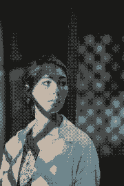 |
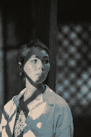 |
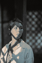 |
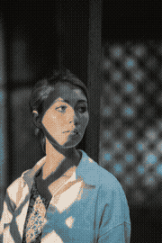 |
We can see the hue timidly appearing around K=16 (specifically it starts
being more strongly noticeable starting the cut K=13).
Conclusion
For now, I'm mostly done with this "week-end long project" into which I actually poured 2 or 3 months of lifetime. The FFmpeg patchset will likely be upstreamed soon so everyone should hopefully be able to benefit from it in the next release. It will also come with additional dithering methods, which implementation actually was a relaxing distraction from all this hardship. There are still many ways of improving this work, but it's the end of the line for me, so I'll trust the Internet with it.