Invert a function using Newton iterations

Newton's method is probably one of the most popular algorithm for finding the roots of a function through successive numeric approximations. In less cryptic words, if you have an opaque function f(x), and you need to solve f(x)=0 (finding where the function crosses the x-axis), the Newton-Raphson method gives you a dead simple cookbook to achieve that (a few conditions need to be met though).

I recently had to solve a similar problem where instead of finding the roots I had to inverse the function. At first glance this may sound like two entirely different problems but in practice it's almost the same thing. Since I barely avoided a mental breakdown in the process of figuring that out, I thought it would make sense to share the experience of walking the road to enlightenment.

A function and its inverse

We are given a funky function, let's say f(x)=2/3(x+1)²-sin(x)-1, and we want to figure out its inverse f¯¹():

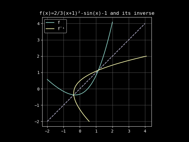
The diagonal is highlighted for the symmetry to be more obvious. One thing you may immediately wonder is how is such an inverse function even possible? Indeed, if you look at x=0, the inverse function gives (at least) 2 y values, which means it's impossible to trace according to the x-axis. What we just did here is we swapped the axis: we simply drew y=f(x) and x=f(y), which means the axis do not correspond to the same thing whether we are looking at one curve or the other. For y=f(x) (abbreviated f or f(x)), the horizontal axis is the x-axis, and for x=f(y) (abbreviated f¯¹ or f¯¹(y)) the horizontal axis is the y-axis because we actually drew the curve according to the vertical axis.

What can we do here to bring this problem back to reality? Well, first of all we can reduce the domain and focus on only one segment of the function where the function can be inverted. This is one of the condition that needs to be met, otherwise it is simply impossible to solve because it doesn't make any sense. So we'll redefine our problem to make it solvable by assuming our function is actually defined in the range R=[R₀,R₁] which we arbitrarily set to R=[0.1;1.5] in our case (could be anything as long as we have no discontinuity):

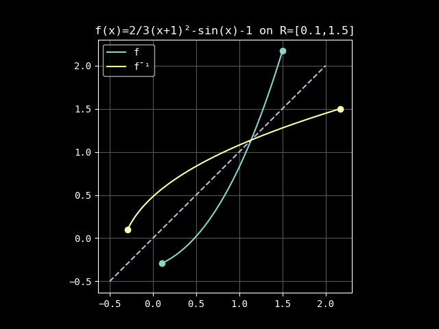
Now f' (the derivative of f) is never null, implying there won't be multiple solution for a given x, so we should be safe. Indeed, while we are still tracing f¯¹ by flipping the axis, we can see that it could also exist in the same space as f, meaning we could now draw it according to the horizontal axis, just like f.

What's so hard though? Bear with me for a moment, because this took me quite a while to wrap my head around. The symmetry is such that it's trivial to go from a point on f to a point on f¯¹:

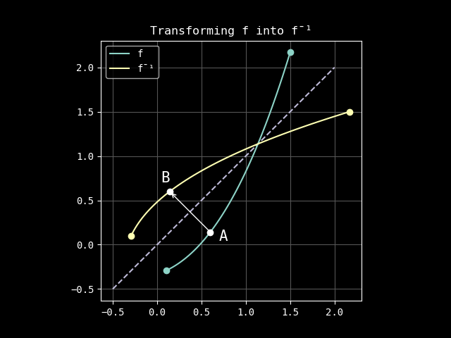
Transforming point A into point B is a matter of simply swapping the coordinates. Said differently, if I have a x coordinate, evaluating f(x) will give me the A.y coordinate, so we have A=(x,f(x)) and we can get B with B=(A.y,A.x)=(f(x),x). But while we are going to use this property, this is not actually what we are looking for in the first place: our input is the x coordinate of B (or the y coordinate of A) and we want the other component.

So how do we do that? This is where root finding actually comes into play.

Root finding

We are going to distance ourselves a bit from the graphic representation (it can be quite confusing anyway) and try to reason with algebra. Not that I'm much more comfortable with it but we can manage something with the basics here.

The key to not getting your mind mixed up in x and y confusion is to use different terms because we associate x and y respectively with the horizontal and vertical axis. So instead we are going to redefine our functions according to u and v. We have:

1. f(u)=v
2. f¯¹(v)=u (reminder: v is our input and u is what we are looking for)

Note: writing f¯¹ doesn't mean our function is anything special, the ¯¹ simply acts as some sort of semantic tagging, we could very well have written h(v)=v. Both functions f and f¯¹ are simply mapping a real number to another one.

In the previous section we've seen than f(u)=v is actually equivalent to f¯¹(v)=u. This may sound like an arbitrary statement, so let me rephrase it differently: for a given value of u it only exists one corresponding value of v. If we now feed that same v to f¯¹ we will get u back. To paraphrase this with algebra: f¯¹(f(u)) = u.

How does that all of this help us? Well it means that f¯¹(v)=u is equivalent to f(u)=v. So all we have to do is solve f(u)=v, or f(u)-v=0. The process of solving this equation to find u is equivalent to evaluating f¯¹(v).

And there we have it, with a simple subtraction of v, we're back into known territory. We declare a new function g(u)=f(u)-v and we are going to find its root by solving g(u)=0 with the help of Newton's method.

Summary with less babble:

f¯¹(v)=u ⬄ f(u)=v
         ⬄ f(u)-v=0
         ⬄ g(u)=0 with g(u)=f(u)-v

Newton's method

The Newton iterations are dead-ass simple: it's a suite (or an iterative loop if you prefer):

uₙ₊₁ = uₙ - g(uₙ)/g'(uₙ)

…repeated as much as needed (it converges quickly).

• g is the function from which we're trying to find the root
• g' its derivative
• u our current approximation, which gets closer to the truth at each iteration

We can evaluate g (g(u)=f(u)-v) but we need two more pieces to the puzzle: g' and an initial value for u.

Derivative

There is actually something cool with the derivative g': since v is a constant term, the derivative of g is actually the derivative of f: g(u)=f(u)-v so g'(u)=f'(u).

This means that we can rewrite our iteration according to f instead of g:

uₙ₊₁ = uₙ - (f(uₙ)-v)/f'(uₙ)

Now for the derivative f' itself we have two choices. If we know the function f, we can derive it analytically. This should be the preferred choice if you can because it's faster and more accurate. In our case:

 f(x) = 2/3(x+1)² - sin(x) - 1
f'(x) = 4x/3 - cos(x) + 4/3

You can rely on the derivative rules to figure the analytic formula for your function or… you can cheat by using "derivative …" on WolframAlpha.

But you may be in the situation where you don't actually have that information because the function is opaque. In this case, you could use an approximation: take a very small value ε (let's say 1e-6) and approximate the derivative with for example f'(x)=(f(x+ε)-f(x-ε))/(2ε). It's a dumb trick: we're basically figuring out the slope by taking two very close points around x. This would also work by using g instead of f, but you have to compute two extra subtractions (the - v) for no benefit because they cancel each others.

Initial approximation

For the 3rd and last piece of the puzzle, the initial u, we need to figure out something more elaborate. The simplest we can do is to start with a first approximation function f₀¯¹ as a straight line between the point (f(R₀),R₀) and (f(R₁),R₁). How do we create a function that linearly link these 2 points together? We of course use one of the most useful math formulas: remap(a,b,c,d,x) = mix(c,d,linear(a,b,x)), and we evaluate it for our first approximation value u₀:

u₀ = remap(f(R₀),f(R₁),R₀,R₁,v)

If your boundaries are simpler, typically if R=[0;1], this expression can be dramatically simplified. A linear() might be enough, or even a simple division. We have a pathological case here so we're using the generic expression.

We get:

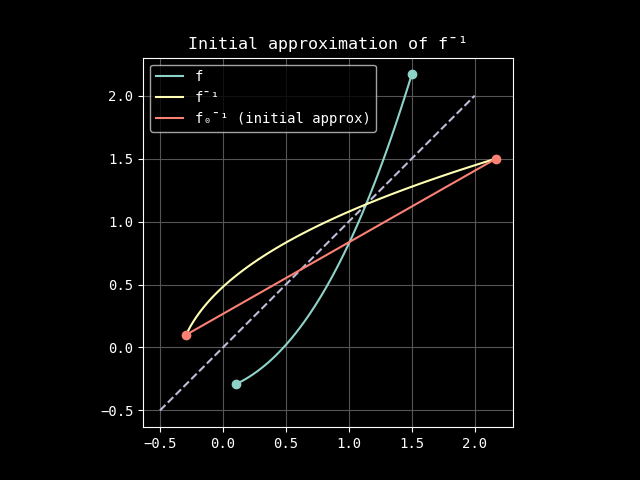
Close enough, we can start iterating from here.

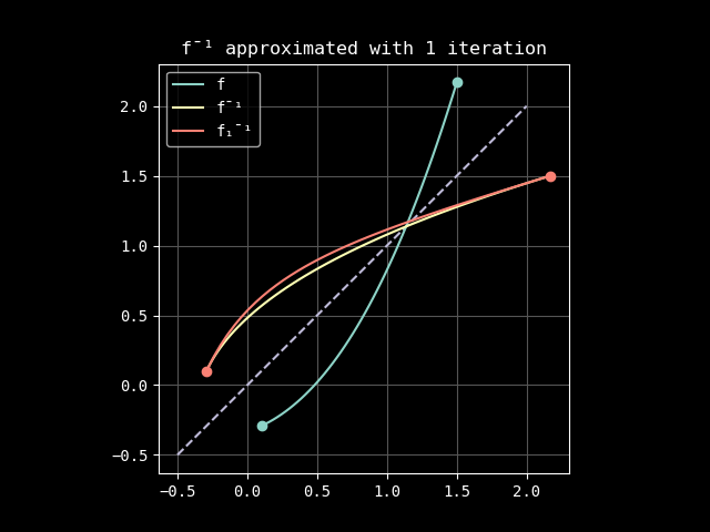
Iterating

If we do a single Newton iteration, u₁ = u₀ - (f(u₀)-v)/f'(u₀) our straight line becomes:

With one more iteration:

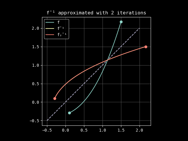
Seems like we're getting pretty close, aren't we?

If you want to converge even faster, you may want to consider Halley's method. It's more expensive to compute, but 1 iteration of Halley may cost less than 2 iterations of Newton. Up to you to study if the trade-off is worth it.

Demo code

If you want to play with this, here is a matplotlib demo generating a graphic pretty similar to what's found in this post:

import numpy as np
import matplotlib.pyplot as plt

N = 1  # Number of iterations
R0, R1 = (0.1, 1.5)  # Reduced domain

# The function to inverse and its derivative
def f(x): return 2 / 3 * (x + 1) ** 2 - np.sin(x) - 1
def d(x): return 4 / 3 * x - np.cos(x) + 4 / 3

# The most useful math functions
def mix(a, b, x): return a * (1 - x) + b * x
def linear(a, b, x): return (x - a) / (b - a)
def remap(a, b, c, d, x): return mix(c, d, linear(a, b, x))

# The inverse approximation using Newton-Raphson iterations
def inverse(v, n):
    u = remap(f(R0), f(R1), R0, R1, v)
    for _ in range(n):
        u = u - (f(u) - v) / d(u)
    return u

def _main():
    _, ax = plt.subplots()

    x = np.linspace(R0, R1)
    y = f(x)
    ax.plot((-1 / 2, 2), (-1 / 2, 2), "--", color="gray")
    ax.plot(x, y, "-", color="C0", label="f")
    ax.plot([R0, R1], [f(R0), f(R1)], "o", color="C0")
    ax.plot(y, x, "-", color="C1", label="f¯¹")

    v = np.linspace(f(R0), f(R1))
    u = inverse(v, N)
    ax.plot(v, u, "-", color="C3", label=f"f¯¹ approx in {N} iteration(s)")
    ax.plot([f(R0), f(R1)], [R0, R1], "o", color="C3")

    ax.set_aspect("equal", "box")
    ax.grid(True)
    ax.legend()
    plt.show()

_main()