Understanding selective coloring in Adobe Photoshop

Photoshop has many interesting color filters, most of them being perfidiously documented such that you can understand how to use them, but can't understand how they work. The selective color filter is one of them, which may be part of the reason a colleague and I decided to implement it as an OpenGL shader in the context of a hackaton at our company in 2015.

After completing the reverse engineering of the filter later that year, I rewrote that code in C and integrated it in the FFmpeg project. This means that you can use Photoshop (or After Effects as far as I know) to find some fancy selective color settings, and apply them on video streams using FFmpeg. The parameters can be transmitted manually as filter parameters, or through a preset file.

This article is meant to detail the (very much simplified) process I went through while reversing the filter, as well as providing all the formulas you need to implement it yourself in your applications without having to read the LGPL code from FFmpeg and comply to its license.

If you are interested in the final formulas more than how it was reversed, you can directly jump to the conclusion.

Selective color from a user perspective

The general concept of the filter is pretty straightforward. You start selecting a range of colors you want to affect:

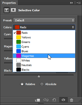
And then you can adjust the value of Cyan, Magenta, Yellow and Black (CMYK) of these affected pixels.

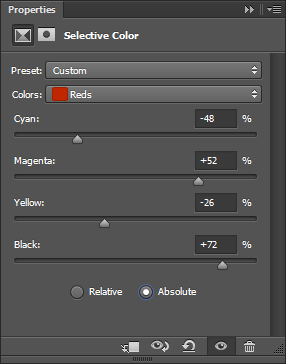
There is then an extra switch for a Relative or Absolute adjustment. We'll clarify this later on, but you can for now consider that Relative is just a scaled down (understand smoother) version of Absolute.

Starting now, I'll refer to Relative and Absolute as "the modes".

Example

Here is a small example with the following settings:

• for Greens, magenta +100%
• for Yellows, yellow -100%
• for Magentas, magenta +50%
• for Blues, yellow -50%

(actually done with -vf "selectivecolor=greens='0 1 0':yellows='0 0 -1':magentas=0 0.5 0:blues=0 0 -0.5")

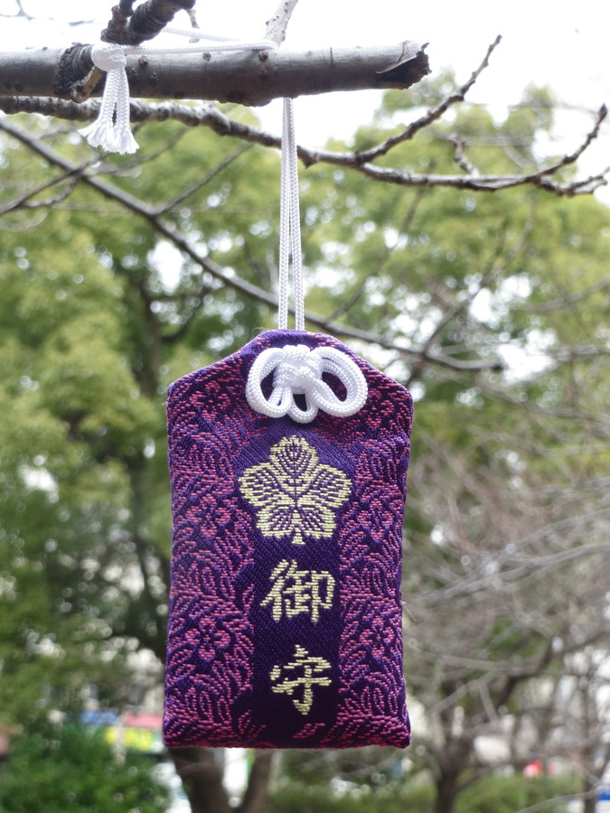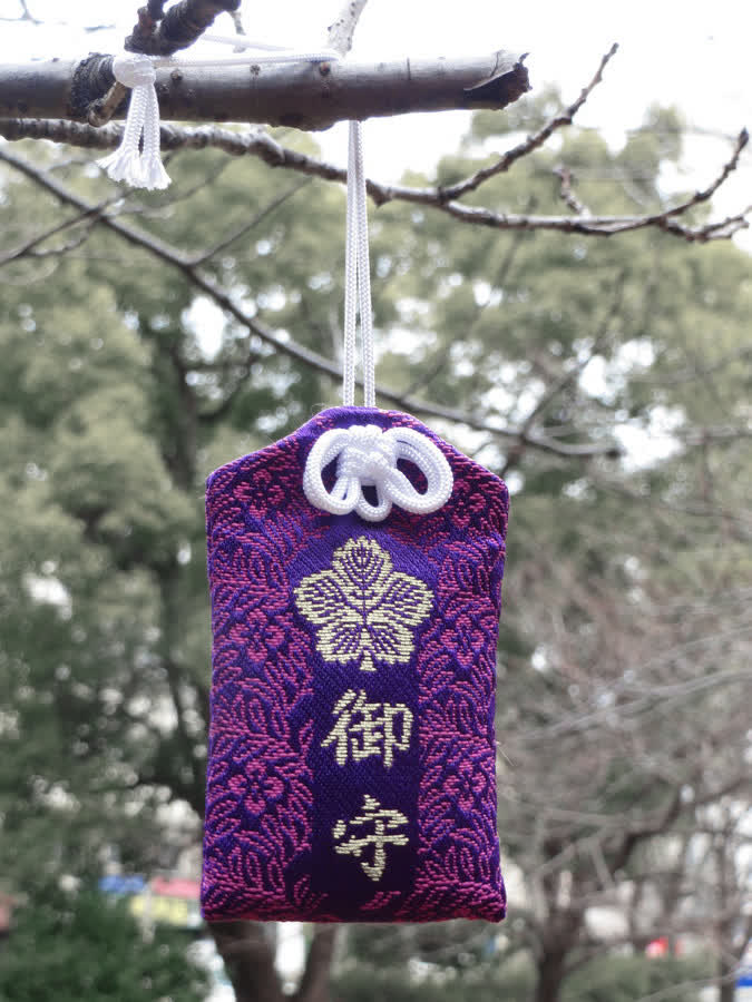Initial observations

By playing with the filter a bit, we can observe the following properties:

• the filter works on a 1:1 pixel basis: the result of the filter applied to a pixel does NOT involve the surrounding pixels. This is good news as it simplifies understanding the filter drastically. As a side note, it also means we have potentially ways to make it fast (threading and direct rendering become straightforward to implement).
• Cyan, Magenta and Yellow sliders are respectively associated with the Red, Green and Blue component of the pixel. This is also interesting as it means we can study components independently: Cyan and Red, Magenta and Green, and Yellow and Blue.
• we can cumulate changes on several ranges simultaneously (for instance making changes to the Reds, to the Whites and to the Yellows). These ranges could overlap.

Mathematical modeling

Based on our observations, we can formalize our filter mathematically with the following:

Note for programmers like me who have a really hard time with math: N is simply the maximum value a component can have. So with a 8-bit depth picture, N=(1<<8)-1=255.

What Internet tells us

I'm not the first one to try to reverse the filter, and it would be dishonest of me to not mention this translated Chinese article on Adobe Selective Color.

Indeed, it actually describes in a lot of details how the filter works, and the first implementation we did was based pretty much solely on it.

But it also has several limitations:

• very confusing on many aspects (probably partly due to the translation)
• the Blacks slider is vaguely mentioned and the explanation actually sounds wrong according to my findings
• the Relative explanation is also, as far as I can tell, inaccurate at best

Still, this article was extremely valuable, and I'll take from it two information which I'll use arbitrarily later:

• the effective ranges of the colors (what are Reds, Yellows, ...)
• the scales formula (I'll talk about them when we will reach them)

These findings could also have been included within this research, but the article would have been much longer, so I'd like to thank the author and the translator for their valuable contribution.

First model adjustment

We have modeled our problem: we need to determine our adjustment function f.

We know only the selected colors are affected, so we can already clarify our model with the following:

• Γ the color classification of the source pixel to compare to the user selection (C)
• v one component value of the source pixel (r, g or b)
• α the corresponding C/M/Y user adjustment value
• φ the actual color component adjustment function

Thanks to the Chinese article we can define how to compute the color classification of the source pixel Γ=T(r,g,b):

Grabbing some data on CMY adjustments

Our goal is now to figure out φ.

Automating pixel data color picking from Photoshop is very annoying. We will try to limit ourselves with not too much data as it will be grabbed manually.

Based on our initial observations, we could start graphing how one pixel color change while affecting every single slider.

We will pick the color (180,100,50) as it is the one used in the Chinese article. This color is classified as a "red" pixel, as in "affected at least by the color range Reds", which is the default range in the filter widget and the one we will select.

Let's try to make C, M and Y vary from -1 to 1 with a relative small step and observe their effect on their corresponding component. Remember, Cyan will only affect the red component of the pixel, Magenta the green, and Yellow the blue.

While at it, we will observe the effect of the modes switch.

Here are the results:

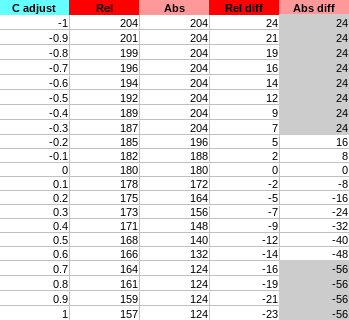
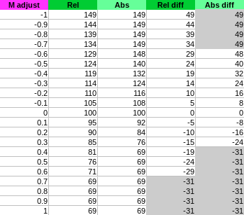
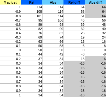
Explanation of the column:

• adjust: user adjustment value of C, M or Y (known as α in our maths)
• Rel: value observed of the corresponding pixel component (R, G or B) in Relative mode
• Abs: value observed of the corresponding pixel component (R, G or B) in Absolute mode
• Rel diff: difference with the original pixel component value in Relative mode
• Abs diff: difference with the original pixel component value in Absolute mode

Since filters can be cumulated we are interested in the difference more than the value itself. Indeed, we want to be able to cumulate multiple different amount of change on the same pixel (if you change the CMYK settings for different overlapping ranges).

This is what graphing Rel diff and Abs diff according to the adjust looks like:

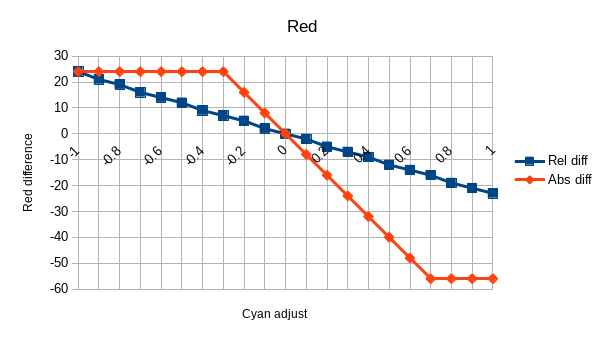
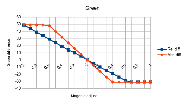
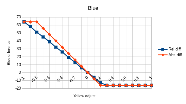
Slope and clipping

It is pretty obvious from these graph that we are facing a linear function (f(x)=ax+b) with an additional clipping.

The clipping also appears to be exactly the same between the modes.

Last notable point: b=0 in f(x)=ax+b. Indeed, in both modes the line is crossing 0 with a value of 0.

From these observations we can already say we have to solve a system such as:

with

• φ() defines the amount to add to the original pixel component value (R, G or B)
• s unknown slope to determine, different between modes
• L and H the clipping boundaries to determine (L for low, H for high)

Since the boundaries are the most visible in Absolute mode, we will focus on it at first.

Slope

With the help of the data we obtain the slope factor easily by solving for example the following systems:

Note: I picked the values as far as possible from zero still not in the clip ranges.

This might not be obvious from the graph because of the different y scale, but in Absolute mode the slope s is indeed exactly the same for all component.

So what is this slope factor s=-80, how does it relate to every information we have so far?

Let's say Ω = -s = 80. Well, our original pixel value is (180,100,50). So it looks like it is simply Ω=r-g. But with more tests we quickly realize the factor is not based on the component position but on its value: Ω = maximum_component - median_component (which is indeed r-g here).

This is the second and last time the Chinese article will help us, this time by providing all the scale factor formulas for the different ranges available:

• S() is the function providing the scale according to the pixel value such that s=-S(r,g,b).
• max(), min() and med() respectively the maximum, minimum and median values

By the way, we can see that S(r,g,b) ≥ 0 in all the scenarios, which means s ≤ 0, or said differently: the slope will always be decreasing like we observe in our graphs.

From now on, to simplify the notation we will consider the source pixel scale Ω = S(r,g,b).

Our φ definition gets improved with the following:

Clipping

We now need to figure out how the clipping values L and H are defined. Given that our boundaries are component specific, we could assume that they depend on its component value, such that:

Well, given all the data we know so far and with trial and error we can pretty quickly figure out that we have the following:

Let's ignore the rounding as we assume it's done on the final adjustment and update our previous system with that clipping information:

Taking Ω out of the clip function we end up with:

Or as an alternative simplified form:

Relative

We know our adjustment function for the Absolute mode, but not yet for the Relative one.

Let's observe the common points and differences between the two:

• same zero origin
• different slope
• apparently the same clipping

From this, we can figure out that we have this scheme:

where x is our unknown. Well, this x is actually a value we already know: the upper boundary, or 1-v/N, so here we go:

Blacks

So far, our formula works with every C, M and Y adjustments in all color ranges and modes. On the other hand, it doesn't handle K (black) yet.

In order to figure out how it influences each component adjustment we will set the C, M, and Y settings to arbitrary constants and observe how the pixel components get adjusted while changing K in the range [-1,1]

We'll pick C=40/100, M=-60/100 and Y=10/100. We will also select the Reds range and pick the same original pixel color of (180,100,50).

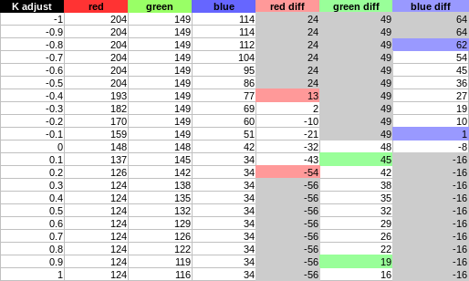
And the graph of the differences according to the K adjustment:

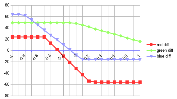
Observations:

• the adjustment is still linear: f(x) = ax+b
• the origin is not 0 like with C, M, Y, which suggest b≠0

That might be good enough to start with, but here is one thing to check: what if, instead of affecting the Reds we would change the Neutrals instead? If you do that experiment, you will realize that the slope and its origin change. This means Ω is likely a factor of both a and b in the linear function.

If we ignore the clipping for now and focus on the line equation first, we get:

Also, our CMY slope s is currently defined by:

We will focus on the Absolute mode where m=1 as it is simpler.

So the results we are observing here are the following:

Using that equation to find out a and b leads to this:

We will assume again the approximation are actually due to the lack of precision in the data and will consider an equality here.

Remember our C, M, and Y values?

So in the end we get:

which we can stick back inside our original formula (Absolute version):

After a quick test, we can see that the m factor from the Relative mode applies on top of this CMYK conversion (which makes perfect sense), so we get:

Conclusion

The entire system can be summed up in the following single picture:

Note about cumulated ranges: we know how to process only a single given range. But if you need to apply different settings to multiple ranges, you just have to sum up all the f() functions computed with a different C setting.