Bézier curves are a core building block of text and 2D shapes rendering. There are several approaches to rendering them, but one especially challenging problem, both mathematically and technically, is computing the distance to a Bézier curve. For quadratic curves (one control point), this is fairly accessible, but for cubic (two control points) we're going to see why it is so hard.
Having this distance field opens up many rendering possibilities. It's hard, but it's possible; here is a live proof:
In this visualization, I'm borrowing your device resources to compute the distance to the curve for every single pixel. The yellow points are the control points of the curve (in white) and the blue zone is a representation of the distance field.
Note
All the demos and code in this article are self-contained GLSL fragment shaders. Most of the code can be found in the article, but feel free to inspect the source code of any of these WebGL demo for the complete code. They can be run verbatim using ShaderWorkshop.
The basic maths
In a previous article, we explained that a Bézier curve can be expressed as a polynomial. In our case, a cubic polynomial:
Where a, b, c and d are the vector coefficients derived from the start (P_0), end (P_3), and control points (P_1, P_2) using the following formulas (you can refer to the previous article for details):
For a given point p in 2D space, the distance to that Bézier curve can be expressed as a length between our curve and p:
Our goal is to find the t value where d(t) is the smallest.
The length formula has an annoying square root, so we start with the distance squared for simplicity, which we are going to unroll:
The derivative of that function will allow us to identify critical points: that is, points where the distance starts growing or reducing. Said differently, solving D'(t)=0 will identify all the maximums and minimums (we're interested in the latter) of D(t) (and thus d(t) as well).
It is a bit convoluted in our case but straightforward to compute:
A polynomial, this time of degree 5, emerges here. For conciseness, we can express D'(t) polynomial coefficients as a bunch of dot products:
Finally, we notice that solving D'(t)=0 is equivalent to solving D'(t)/2 = 0, so we simplify the expression:
Assuming we are able to solve this equation, we will get at most 5 values of t, among which we should find the shortest distance from p to the curve. Since t is bound within 0 and 1 (start and end of the curve), we will also have to test the distance at these locations.
Note
We could also compute the 2nd derivative in order to differentiate minimums from maximums, but simply evaluating the 5(+2) potential t values and keeping the smallest works just fine.
The red dot in the blue field is a random point in space. The red lines show which distances are evaluated (at most 5+2) to find the smallest one.
Translated to GLSL code
Transposing these formulas into code gives us this base template code:
float bezier_distance(vec2 p, vec2 p0, vec2 p1, vec2 p2, vec2 p3) {
    // Start by testing the distance to the boundary points at t=0 (p0) and t=1 (p3)
    vec2 dp0 = p0 - p,
         dp3 = p3 - p;
    float dist = min(dot(dp0, dp0), dot(dp3, dp3));

    // Bezier cubic points to polynomial coefficients
    vec2 a = -p0 + 3.0*(p1 - p2) + p3,
         b = 3.0 * (p0 - 2.0*p1 + p2),
         c = 3.0 * (p1 - p0),
         d = p0;

    // Solve D'(t)=0 where D(t) is the distance squared
    vec2 dmp = d - p;
    float da = 3.0 * dot(a, a),
          db = 5.0 * dot(a, b),
          dc = 4.0 * dot(a, c) + 2.0 * dot(b, b),
          dd = 3.0 * (dot(a, dmp) + dot(b, c)),
          de = 2.0 * dot(b, dmp) + dot(c, c),
          df = dot(c, dmp);

    float roots[5];
    int count = root_find5(roots, da, db, dc, dd, de, df);
    for (int i = 0; i < count; i++) {
        float t = roots[i];
        // Evaluate the distance to our point p and keep the smallest
        vec2 dp = ((a * t + b) * t + c) * t + dmp;
        dist = min(dist, dot(dp, dp));
    }

    // We've been working with the squared distance so far, it's time to get its
    // square root
    return sqrt(dist);
}
Note
dot(dp,dp) is a shorthand for the length squared, of course cheaper than
computing length() which contains a square root.
Warning
We assume here the root finder only returns the roots that are within [0,1].
root_find5() is our 5th degree root finder, that is the function that gives us
all the t (at most 5) which satisfy:
But before we are able to solve that, we need to study the simpler 2nd degree polynomial solving:
Solving quadratic polynomial equations
Diving into the rabbit hole of solving polynomial numerically will lead you to insanity. But we still have to scratch the surface because superior degree solvers usually rely on it.
My favorite quadratic root finding formula is the super simple one introduced by 3Blue1Brown, which involves locating a mid point m from which you get the 2 surrounding roots r:
In GLSL, a code to cover most common corner cases would look like this:
// Return true if x is not a NaN nor an infinite
// highp is probably mandatory to force IEEE 754 compliance
bool isfinite(highp float x) { return (floatBitsToUint(x) & 0x7f800000u) != 0x7f800000u; }

// Quadratic: solve ax²+bx+c=0
int root_find2(out float r[5], float a, float b, float c) {
    int count = 0;
    float m = -b / (2.*a);
    float d = m*m - c/a;
    if (!isfinite(m) || !isfinite(d)) { // a is (probably) too small
        // Linear: solve bx+c=0
        float s = -c / b;
        if (isfinite(s))
            r[count++] = s;
        return count;
    }
    if (d < 0.) // no root
        return count;
    if (d == 0.) {
        r[count++] = m; // single root
        return count;
    }
    float z = sqrt(d);
    r[count++] = m - z;
    r[count++] = m + z;
    return count;
}
Not quite as straightforward as the math formula, isn't it?
We cannot know in advance whether the division is going to succeed, so we do run divisions and only then check if they failed (and assume a reason for the failing). This is much more reliable than an arbitrary epsilon value. We also try to avoid duplicated roots.
Note
The roots are automatically sorted because z is always positive.
Warning
isfinite() may not be as reliable because in GLSL "NaNs are not required
to be generated", meaning some edge case may not be supported depending on
the hardware, drivers, and the current weather in Yokohama.
As much as I like it, this implementation might not be the most stable numerically (even though I don't have have strong data to back this claim). Instead, we may prefer the formula from Numerical Recipes:
Leading to the following alternative implementation:
int root_find2(out float r[5], float a, float b, float c) {
    int count = 0;
    float d = b*b - 4.*a*c;
    if (d < 0.)
        return count;
    if (d == 0.) {
        float s = -.5 * b / a;
        if (isfinite(s))
            r[count++] = s;
        return count;
    }
    float h = sqrt(d);
    float q = -.5 * (b + (b > 0. ? h : -h));
    float r0 = q/a, r1 = c/q;
    if (isfinite(r0)) r[count++] = r0;
    if (isfinite(r1)) r[count++] = r1;
    return count;
}
This is not perfect at all (especially with the b²-4ac part). There
are actually many other possible implementations, and this HAL CNRS
paper shows how near impossible it is to make a correct one. It is
an interesting but depressing read, especially since it "only" covers IEEE
754 floats, and we have no such guarantee on GPUs. We also don't have fma() in
WebGL, which greatly limits improvements. For now, it will have to do.
Solving quintic polynomial equations: attempt 1
Solving polynomials of degree 5 cannot be solved analytically like quadratics. And even if they were, we probably wouldn't do it because of numerical instability. Typically, in my experience, analytical 3rd degree polynomials solver do not provide reliable results.
The first iterative algorithm I picked was the Aberth–Ehrlich method. Nowadays, more appropriate algorithms exist, but at the time I started messing up with these problems (several years ago), it was a fairly good contender. This video explores how it works.
The convergence to the roots is quick, and it's overall simple to implement. But it's not without flaws. The main problem is that it works in complex space. We can't ignore the complex roots because they all "respond" to each others. And filtering these roots out at the end implies some unreliable arbitrary threshold mechanism (we keep the root only when the imaginary part is close to 0).
The initialization process also annoyingly requires you to come up with a guess at what the roots are, and doesn't provide anything relevant. Aberth-Ehrlich works by refining these initial roots, similar to a more elaborate Newton iterations algorithm. Choosing better initial estimates leads to a faster convergence (meaning less iterations).
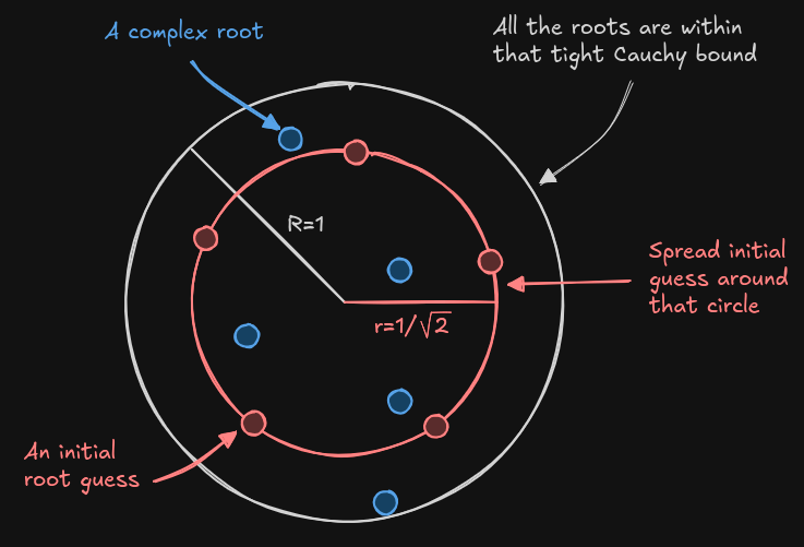
The Cauchy bound specifies a space by defining the radius of a disk (complex
numbers are in 2D space) where all the roots of a polynomial should lie within.
We are going to use it for the initial guess, and more specifically its "tight"
version (which unfortunately relies on pow()).
Since Aberth-Ehrlich is a refinement and not just a shrinking process, we define and use an inner disk that has half the area of Cauchy bound disk. That way, we're more likely to start with initial guesses spread in the "middle" of the roots; this is where the √2 comes from in the formula below.
#define K5_0 vec2( 0.951056516295154,  0.309016994374947)
#define K5_1 vec2( 0.000000000000000,  1.000000000000000)
#define K5_2 vec2(-0.951056516295154,  0.309016994374948)
#define K5_3 vec2(-0.587785252292473, -0.809016994374947)
#define K5_4 vec2( 0.587785252292473, -0.809016994374948)

int root_find5_aberth(out float roots[5], float a, float b, float c, float d, float e, float f) {
    // Initial candidates set mid-way of the tight Cauchy bound estimate
    float r = (1.0 + max_5(
        pow(abs(b/a), 1.0/5.0),
        pow(abs(c/a), 1.0/4.0),
        pow(abs(d/a), 1.0/3.0),
        pow(abs(e/a), 1.0/2.0),
            abs(f/a))) / sqrt(2.0);

    // Spread in a circle
    vec2 r0 = r * K5_0,
         r1 = r * K5_1,
         r2 = r * K5_2,
         r3 = r * K5_3,
         r4 = r * K5_4;
The circle constants are generated with the following script:
import math
import sys

n = int(sys.argv[1])
for k in range(n):
    angle = 2 * math.pi / n
    off = math.pi / (2 * n)
    z = angle * k + off
    c, s = math.cos(z), math.sin(z)
    print(f"#define K{n}_{k} vec2({c:18.15f}, {s:18.15f})")
Next, it's basically a simple iterative process. Unrolling everything for degree 5 looks like this:
#define close_to_zero(x) (abs(x) < eps)

// This also filters out roots out of the [0,1] range
#define ADD_ROOT_IF_REAL(r) if (close_to_zero(r.y) && r.x >= 0. && r.x <= 1.) roots[count++] = r.x

#define SMALL_OFF(off) (dot(off, off) <= eps*eps)

/* Complex multiply, divide, inverse */
vec2 c_mul(vec2 a, vec2 b) { return mat2(a, -a.y, a.x) * b; }
vec2 c_div(vec2 a, vec2 b) { return mat2(a, a.y, -a.x) * b / dot(b, b); }
vec2 c_inv(vec2 z)         { return vec2(z.x, -z.y) / dot(z, z); }

// Compute f(x)/f'(x): complex polynomial evaluation (y) divided by their
// derivatives (q) using Horner's method in one pass
vec2 c_poly5d4(float a, float b, float c, float d, float e, float f, vec2 x) {
    vec2 y =       a*x  + vec2(b, 0), q =       a*x  + y;
         y = c_mul(y,x) + vec2(c, 0); q = c_mul(q,x) + y;
         y = c_mul(y,x) + vec2(d, 0); q = c_mul(q,x) + y;
         y = c_mul(y,x) + vec2(e, 0); q = c_mul(q,x) + y;
         y = c_mul(y,x) + vec2(f, 0);
    return c_div(y, q);
}

vec2 sum_of_inv(vec2 z0, vec2 z1, vec2 z2, vec2 z3, vec2 z4) { return c_inv(z0 - z1) + c_inv(z0 - z2) + c_inv(z0 - z3) + c_inv(z0 - z4); }

int root_find5_aberth(out float roots[5], float a, float b, float c, float d, float e, float f) {
    if (close_to_zero(a))
        return root_find4_aberth(roots, b, c, d, e, f);

    // Code snip: see previous snippet
    // float r = ...
    // vec2 r0, r1, r2, ...

    for (int m = 0; m < 16; m++) {
        vec2 d0 = c_poly5d4(a, b, c, d, e, f, r0),
             d1 = c_poly5d4(a, b, c, d, e, f, r1),
             d2 = c_poly5d4(a, b, c, d, e, f, r2),
             d3 = c_poly5d4(a, b, c, d, e, f, r3),
             d4 = c_poly5d4(a, b, c, d, e, f, r4);

        vec2 off0 = c_div(d0, vec2(1,0) - c_mul(d0, sum_of_inv(r0, r1, r2, r3, r4))),
             off1 = c_div(d1, vec2(1,0) - c_mul(d1, sum_of_inv(r1, r0, r2, r3, r4))),
             off2 = c_div(d2, vec2(1,0) - c_mul(d2, sum_of_inv(r2, r0, r1, r3, r4))),
             off3 = c_div(d3, vec2(1,0) - c_mul(d3, sum_of_inv(r3, r0, r1, r2, r4))),
             off4 = c_div(d4, vec2(1,0) - c_mul(d4, sum_of_inv(r4, r0, r1, r2, r3)));

        r0 -= off0;
        r1 -= off1;
        r2 -= off2;
        r3 -= off3;
        r4 -= off4;

        if (SMALL_OFF(off0) && SMALL_OFF(off1) && SMALL_OFF(off2) && SMALL_OFF(off3) && SMALL_OFF(off4))
            break;
    }

    int count = 0;
    ADD_ROOT_IF_REAL(r0);
    ADD_ROOT_IF_REAL(r1);
    ADD_ROOT_IF_REAL(r2);
    ADD_ROOT_IF_REAL(r3);
    ADD_ROOT_IF_REAL(r4);
    return count;
}
When the main coefficient is too small, we fall back on the 4th degree (and so on until we reach the analytic quadratic). The 4th and 3rd degree versions of this function are easy to guess (they're pretty much identical, just removing one coefficient at each degree).
We're also hardcoding a maximum of 16 iterations here because it's usually enough. To have an idea of how many iterations are required in practice, following is a visualization of the heat map of the number of iterations for every pixel:
The big picture and the weaknesses of the algorithm should be pretty obvious by now. Among all drawbacks of this approach, there are also surprising pathological cases where the algorithm is not performing well. Fortunately, there were some progress on the state of the art in recent years.
Solving quintic polynomial equations: the state of the art
In 2022, Cem Yuksel published a new algorithm for polynomial root solving. Initially I had my reservations because the official implementation had a few shortcomings on some edge cases, which made me question its reliability. It's also optimized for CPU computation and is, to my very personal taste, overly complex.
Fortunately, Christoph Peters showed that it was possible on the GPU by implementing it for very large degrees, and without any recursion. Inspired by that, I decided to unroll it myself for degree 5.
One core difference with Aberth approach is that it is designed for arbitrary ranges. In our case this is actually convenient because, due to how Bézier curves are defined, we are only interested in roots between 0 and 1. We will need to adjust the Quadratic function to work in this range, as well as keeping the roots ordered:
     }
     float h = sqrt(d);
     float q = -.5 * (b + (b > 0. ? h : -h));
-    float r0 = q/a, r1 = c/q;
-    if (isfinite(r0)) r[count++] = r0;
-    if (isfinite(r1)) r[count++] = r1;
+    vec2 v = vec2(q/a, c/q);
+    if (v.x > v.y) v.xy = v.yx; // keep them ordered
+    if (isfinite(v.x) && v.x >= 0. && v.x <= 1.) r[count++] = v.x;
+    if (isfinite(v.y) && v.y >= 0. && v.y <= 1.) r[count++] = v.y;
     return r;
 }
The core logic of the algorithm relies on a cascade of derivatives for every degree. Christoph Peters provides an analytic formula to obtain the derivative for any degree. This is a huge helper when we need to work for an arbitrary degree, but in our case we can just differentiate manually:
Since we're only interested in the roots, similar to what we did to D(t), we can simplify some of these expressions:
The purpose of that cascade of derivatives is to cut the curve into monotonic segments. In practice, the core function looks like this:
int root_find5_cy(out float r[5], float a, float b, float c, float d, float e, float f) {
    float r2[5], r3[5], r4[5];
    int n = root_find2(r2,          10.*a, 4.*b,    c);            // degree 2
    n = cy_find5(r3, r2, n, 0., 0., 10.*a, 6.*b, 3.*c,   d);       // degree 3
    n = cy_find5(r4, r3, n,     0.,  5.*a, 4.*b, 3.*c, d+d, e);    // degree 4
    n = cy_find5(r,  r4, n,             a,    b,    c,   d, e, f); // degree 5
    reutnr n;
}
We could unroll cy_find3, cy_find4, and cy_find5, but to keep the
code simple, the degree 3 to 5 will share the same function, with leading
coefficients set to 0 (hopefully the compiler does its job properly).
cy_find5 relies on roots found (at most 4) at previous stages to define
intervals of search:
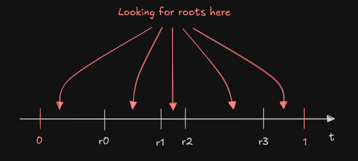
Such an approach has the nice side effect of keeping the roots ordered.
The solver itself is not that complex either:
float poly5(float a, float b, float c, float d, float e, float f, float t) {
     return ((((a * t + b) * t + c) * t + d) * t + e) * t + f;
}

// Quintic: solve ax⁵+bx⁴+cx³+dx²+ex+f=0
iint cy_find5(out float r[5], float r4[5], int n, float a, float b, float c, float d, float e, float f) {
    int count = 0;
    vec2 p = vec2(0, poly5(a,b,c,d,e,f, 0.));
    for (int i = 0; i <= n; i++) {
        float x = i == n ? 1. : r4[i],
              y = poly5(a,b,c,d,e,f, x);
        if (p.y * y > 0.)
            continue;
        float v = bisect5(a,b,c,d,e,f, vec2(p.x,x), vec2(p.y,y));
        r[count++] = v;
        p = vec2(x, y);
    }
    return count;
}
The last brick of the algorithm is the Newton bisection, the slowest part:
// Newton bisection
//
// a,b,c,d,e,f: 5th degree polynomial parameters
// t: x-axis boundaries
// v: respectively f(t.x) and f(t.y)
float bisect5(float a, float b, float c, float d, float e, float f, vec2 t, vec2 v) {
    float x = (t.x+t.y) * .5; // mid point
    float s = v.x < v.y ? 1. : -1.; // sign flip
    for (int i = 0; i < 32; i++) {
        // Evaluate polynomial (y) and its derivative (q) using Horner's method in one pass
        float y = a*x + b, q = a*x + y;
              y = y*x + c; q = q*x + y;
              y = y*x + d; q = q*x + y;
              y = y*x + e; q = q*x + y;
              y = y*x + f;

        t = s*y < 0. ? vec2(x, t.y) : vec2(t.x, x);
        float next = x - y/q; // Newton iteration
        next = next >= t.x && next <= t.y ? next : (t.x+t.y) * .5;
        if (abs(next - x) < eps)
            return next;
        x = next;
    }
    return x;
}
And that's pretty much it. Looking at its heat map, it has a completely different look than Aberth:
The number of iterations might be larger but it is much faster (I observed a factor 3 on my machine), the code is shorter, and actually more reliable.
Note
The scale used to represent the heat map is not the same as the one used in Aberth, but it is identical with the method presented in the next section.
Exploring ITP convergence
The bisection being the hot loop, it is interesting to ponder how to make this faster. A while back, Raph Levien hypothesized about how the ITP method could perform. Out of curiosity, I gave it a chance. The function is designed to work like a bisection, claiming to be as performant in the worst case.
There isn't a lot of code, and the paper provides a pseudo-code. But implementing it was actually challenging in many ways.
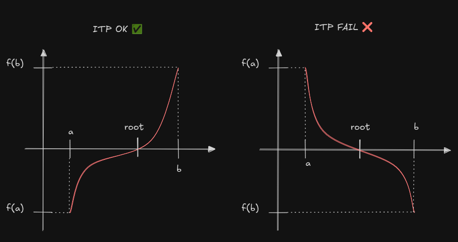
First of all, the authors didn't seem to find relevant to mention that it only works if f(a)<0<f(b). If f(a)>0>f(b), you're pretty much on your own. It requires just 2 lines of adjustments but figuring out this shortcoming of the algorithm was particularly unexpected.
Another bothering aspect concerns the parameters: K_1, K_2 and n_0. The paper proposes those:
I played with them for a while and couldn't find any set that would make a real difference, so I ended up with the following:
- For performance reasons, reducing K_2 to a value of 2 saves a call to
pow(). - For K_1, CRAN seems to suggest \frac{0.2}{b-a} so I went along with it
- And for n_0, well 1 or 2 seem to be the usual parameter.
In the end, the function looks like this:
// ITP algorithm (2020) by Oliveira & Takahashi
// "An Enhancement of the Bisection Method Average Performance Preserving Minmax Optimality"
//
// a,b,c,d,e,f: 5th degree polynomial parameters
// t: x-axis boundaries (a and b in the paper)
// v: respectively f(a) and f(b) in the paper (evaluation of the function with t.x and t.y)
float itp5(float a, float b, float c, float d, float e, float f, vec2 t, vec2 v) {
    float diff = t.y-t.x;

    // K1 and n0 suggested by CRAN
    float K1 = .2 / diff;
    int n0 = 1;

    // The paper has the assumption that f(a)<0<f(b) but we want to
    // support f(a)>0>f(b) too, so we keep a sign flip
    float s = v.x < v.y ? 1. : -1.;

    // Using log(ab)=log(a)+log(b): log2(x/(2ε)) <=> log2(x/ε)-1
    int nh = int(ceil(log2(diff/eps)-1.)); // n_{1/2} (half point)
    int n_max = nh + n0;

    // ε 2^(n_max-k) = ε 2^n_max 2^-k = ε 2^n_max ½^k
    // ½^k is done iteratively in the loop, simplifying the arithmetic
    float q = eps * float(1<<n_max);

    while (diff > eps+eps) {
        // Interpolation
        float xf = (v.y*t.x - v.x*t.y) / (v.y-v.x); // Regula-Falsi

        // Truncation
        float xh = (t.x+t.y) * .5; // x half point
        float sigma = sign(xh - xf);
        float delta = K1*diff*diff; // save a pow() by forcing K2=2
        float xt = delta <= abs(xh - xf) ? xf + sigma*delta : xh; // xt: truncation of xf

        // Projection
        float r = q - diff*.5;
        float x = abs(xt-xh) <= r ? xt : xh-sigma*r;

        // Updating
        float y = poly5(a,b,c,d,e,f, x);
        float side = s*y;
        if      (side > 0.) t.y=x, v.y=y;
        else if (side < 0.) t.x=x, v.x=y;
        else                return x;

        diff = t.y-t.x;
        q *= .5;
    }
    return (t.x+t.y) * .5;
}
This function can be used as a drop'in replacement for bisect5.
I had a lot of expectations about it, but in the end it requires more iterations
than the bisection we implemented. The paper claims to perform at least as good
as a bisection, but our bisect5 is driven by the derivatives so it converges
much faster. Here is the heat map with itp5 instead of bisect5:
Conclusion
The naive unrolled version of Cem Yuksel paper definitely is, so far, the best choice for our problem. I have still concerns about how to implement a good quadratic formula, and I have my reservations about various edge cases. There is also still room for improvements in the cubic solver (degree 3) because it's still a special case where analytical formulas exist, but in general this implementation is satisfying.
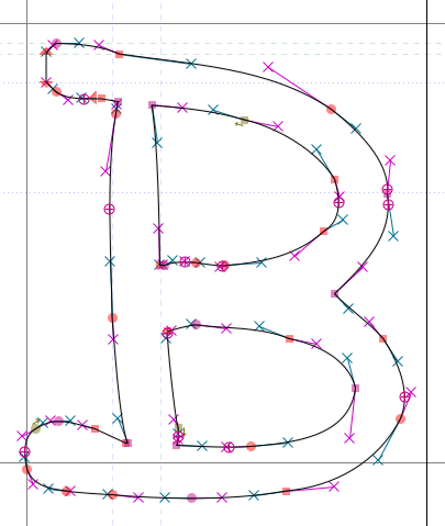
The next step is to work with chains of Bézier curves to make up complex shapes (such as font glyphs). It will lead us to build a signed distance field. This is not trivial at all and mandates one or several dedicated articles. We will hopefully study these subjects in the not-so-distant future.