Code golfing a tiny demo using maths and a pinch of insanity

A few weeks ago, I made a tiny demo that fits into 464 characters:

void main(){vec3 c,p,K=vec3(3,1,0);for(float i,a,g=1.,t,h,d,w,k=.15;i++<1e2;d=
max(max(d-3.,-d),0.)*k,w=g-g*exp(-mix(h*3e2,d*2.5,a=h<.001?0.:1.)),g-=w*a,c+=w*
a*d*9.+(d==0.?K*.01*h:c-c),a=min(p.y+2.,1.),c.r+=w*a*a*.2,t+=min(h*.2,k*=1.015)
,p=normalize(vec3(P+P-R,R.y))*t,p.xz*=mat2(cos(sin(T*.2)+K.zyxz*11.)),p.z+=T*.3
)for(d=p.y,h=d+.5,a=.01;a<1.;a+=a)p.xz*=mat2(8,6,-6,8)*.1,d+=abs(dot(sin((p/a+T
)*.3),p/p))*a,h+=abs(dot(sin(p.xz*.6/a),P/P))*a;O=vec4(tanh(c*.5),1);}

There is no texture, no mesh, no 3D helper: it's simply a procedural mathematical formula evaluated at each pixel assigning them a color. Code golfing is about making it as short as possible, and thus is part of the art performance.

To put things into perspective, the 853x480 JPEG thumbnail of this article is 162x larger than this code.

You can watch a larger version on its main dedicated page, or a portage on Shadertoy (508 chars). If your device is not powerful enough (I'm sorry for the lag on this page) or doesn't support WebGL2, a short preview video (of a slightly outdated variant) can be seen on Mastodon.

I'm guessing the wizardry of the code has confused many people so we're going to dive through the making-of together. Overall, this demo is a particularly dense and entangled compilation of different techniques, where each aspect could mandate a dedicated article. For that reason, some parts will prefer to link to external resources when the literacy is verbose on the subject.

The base template

The code is written in GLSL and is executed for each pixel (technically each fragment) on a simple quad geometry (to be accurate it's even a single big triangle). There is no geometry aside from that, it's basically just a fragment shader.

The fragment receives 3 different inputs:

• the canvas resolution vec2 R
• the time float T
• the pixel position vec2 P (basically gl_FragCoord.xy)

And it has to output a sRGB color in out vec3 O. The code has to be written in a void main() function, and that's pretty much all we need to start.

If you're curious about the glue to setup WebGL2, just look at the source code on the dedicated page. There is no external dependency and the canvas setup code is pretty simple.

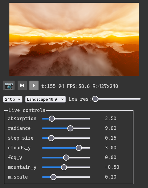
Development setup

For development, people usually directly use Shadertoy. I prefer to use my own local live coding environment: ShaderWorkshop. It can be run without setting up anything, just uv run --with shader-workshop sw-server (assuming the uv Python package manager is installed on the machine). Aside from the comfort of being able to use your favorite code editor, it allows instancing live controls for uniforms very easily, making it smooth to interact with any value and get an immediate feedback.

Noise

One of the core primitive we need is a noise function: it is required for the mountains, the fog, and the clouds.

In a recent article, I talked about gradient noise. We could technically use that, but it will have a lot of drawbacks. First of all, it's super expensive. I know because I made a demo using it the other day, and it was awfully slow. Once per pixel would be fine, but in our case it will have to be evaluated a hundred times, so we need something faster.

Secondly, we're trying to make it as short as possible, and the 2D gradient noise, even minified, is already twice as big as the size of the full demo. We will also need a 3D noise for the clouds and fog, which is even larger and more expensive. And that's not even accounting for the fbm signal combination code.

Inigo Quilez, in his famous Rainforest, used value noise. It is faster, but it still won't do for us for the same reasons, just somehow mitigated. And since we're professionals, we're not going to cheat by sampling a noise texture.

Fortunately, while reverse engineering some Shadertoy demos, in particular the ones from diatribes, I came across some code that made use of this incredible technique of accumulating sine waves.

Combining sin waves

Let's say we want to combine two sine waves in order to get a height map as a 3rd dimension. There are multiple ways of achieving that. For example, we can multiply them:

But we could also add them together:

The surprising take here is that... it's pretty much equivalent. It doesn't give the same result for sure, but visually it could be considered the same, just with a frequency and amplitude a bit different, and rotated on the z axis by 45°.

Similarly, you may think using cosines instead of sinusoids would make a difference, but no, even when combined together, they always give the same base pattern we just saw.

So let's pick one, let's say z=\sin x + \sin y. But this time, we're going to take the absolute value to transform the up and down pattern into bumps:

These bumps are the perfect base for clouds, but not so much for spiky mountains going through aggressive erosion. But with the help of this weird little trick, we can just flip the shape upside down to get sharp edges:

We now have the basis for both our clouds and mountains, but it's not yet convincing. The next step is to use the fbm loop as if we were dealing with Gaussian or value noise: we accumulate several frequencies of our signal together:

• S is the sign (-1 for spiky, 1 for bobby)
• i is the octave identifier going from 0 to N-1 (included).
• F(x,y) is usually the noise signal function, in our case it's the sinusoid combination function, we choose |\sin x + \sin y| here.
• l is the lacunarity factor, that is how frequency changes at each octaves; this is usually a multiply by 2 or a close value.
• g is the gain, that is by how the amplitude changes at each octaves; this is usually a multiply by 0.5 or a close value.

Without surprise this is still very periodic, but we can see a glimpse of chaos emerging. The final touch does all the magic: all we have to do now is simply rotate each layer by like, 30° or something (I'll pick 0.5 radians here, or about 29°):

The symmetry around the origin is still noticeable, but the illusion will work as we will move away from it. It's also possible to add some phase or offsetting (arbitrary addition within the sin or between each layer).

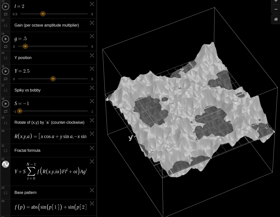
I implemented this in a Desmos 3D scene with all the parameters if one wants to play with it. The formula there has a few more controls, for example the vertical location, an optional transition offset in addition to the rotation, and controls for the base frequency and amplitude.

If this mathematical gibberish is above your head, a GLSL code for the 2D noise could look like this with a lacunarity of 2, a gain of 0.5 and 5 octaves:

float noise(vec2 p) {
    float v = 0.0;
    float amplitude = 1.0;
    for (int i = 0; i < 5; i++) {
        p = rotate(0.5) * p; // rotate our space (more on this in the next section)
        v += abs(sin(p.x) + sin(p.y)) * amplitude; // accumulate noise
        p *= 2.0; // double the frequency at each octave
        amplitude *= 0.5; // half the amplitude at each octave
    }
    return v;
}

One cool trick here: abs(sin(p.x)+sin(p.y)) could also be written abs(dot(sin(p),vec2(1))). This is interesting because now we can operate on the two components of p, easing the possibility to modify them at once (for example doing p*A+B). The dot trick doesn't work with sin(p.x)*sin(p.y), but fortunately, as we saw before, multiply and addition are similar and could be swapped in various situations.

Rotations

We needed some rotation for the noise, and they will be required again soon, so we need to have a closer look to them. Let's start with the formula most people are familiar with:

A matrix can be seen as a function, so mathematically writing p'=M \cdot p would be equivalent to the code p=rotate(angle)*p with:

// Matrix for a counter-clockwise rotation
mat2 rotate(float a) {
    return mat2(
        cos(a), sin(a), // column 1
       -sin(a), cos(a)  // column 2
    );
}

Doing p'=M \cdot p is rotating the space p lies into, which means it gives the illusion the object is rotating clockwise. Though, in the expression p=rotate(angle)*p, I can't help but be bothered by the redundancy of p, so I would prefer to write p*=rotate(angle) instead. Since matrices are not commutative, this will instead do a counter-clockwise rotation of the object. The inlined rotation ends up being:

p *= mat2(cos(a),sin(a),-sin(a),cos(a)); // counter-clockwise rotation of object at point p

This is problematic though: we need to repeat the angle 4 times, which can be particularly troublesome if we want to create a macro and/or don't want an intermediate variable for the angle. But I got you covered: trigonometry has a shitton of identities, and we can express every sin according to a cos (and the other way around).

For example, here is another formulation of the same expression:

p *= mat2(cos(a + vec4(0,3,1,0)*PI/2.0));

Now the angle appears only once, in a vectorized cosine call.

GLSL has degrees() and radians() functions, but it doesn't expose anything for \pi nor \tau constants. And of course, it doesn't have sinpi and cospi implementation either. So it's obvious they want us to use \arccos(-1) for \pi and \arccos(0) for \pi/2:

p *= mat2(cos(a + vec4(0,3,1,0)*acos(0.)));

On his Unofficial Shadertoy blog, Fabrice Neyret goes further and provide us with a very cute approximation, which is the one we will use:

p *= mat2(cos(a + vec4(0,11,33,0)));

I checked for the best numbers in 2 digits, and I can confirm they are indeed the ones providing the best accuracy.

On this last figure, the slight red/green on the outline of the circle represents the loss of precision.

This is good when we want a dynamic rotation angle (we will need that for the camera panning typically), but sometimes we just need a hardcoded value: for example in the rotate(0.5) of our combined noise function.

mat2(cos(.5+vec4(0,11,33,0))) is fine but we can do better. Through Inigo's demos I found the following: mat2(.8,.6,-.6,.8). It makes a rotation angle of about 37° (around 0.64 radians) in a very tiny form. Since 0.5 was pretty much arbitrary, we can just use this matrix as well. And we can make it even smaller (thank you jolle):

p *= mat2(8,6,-6,8)*.1; // rotate p counter-clockwise by about 37° without any trigo

One last rotation tip from Fabrice's bag of tricks: rotating in 3D around an axis can be done with the help of GLSL swizzling:

p.xz *= rotate(0.5); // 3D rotation around y-axis (the absent component)

We will use this too.

Camera (and axis) setup

One last essential before going creative is the camera setup.

We start with the 2D P pixel coordinates which we are going to make resolution independent by transforming them into a traditional mathematical coordinates system:

// 1:1 ratio with [-1,1] along the shortest axis (horizontal or vertical)
vec2 u = (2.0*P - R) / min(R.x, R.y);

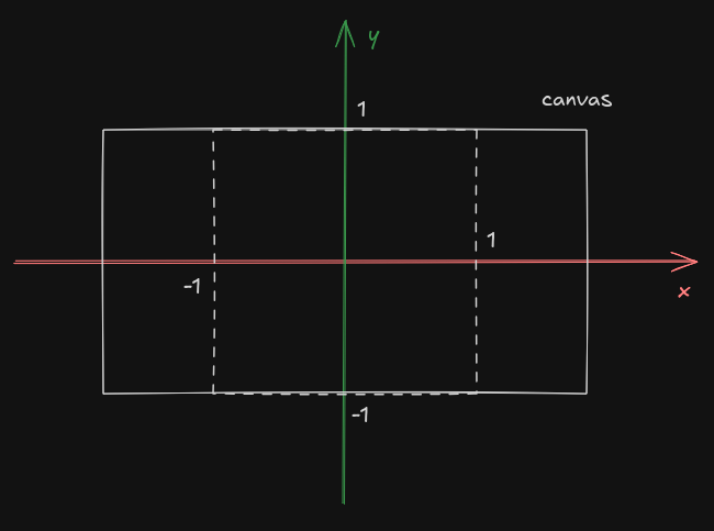
Since we know our demo will be rendered in landscape mode, dividing by R.y is enough. We can also save one character using P+P:

// 1:1 ratio with [-1,1] along the vertical axis
vec2 u = (P+P - R) / R.y;

To enter 3D space, we append a third component, giving us either a right or a left-handed Y-up coordinates system. This choice is not completely random.

Indeed, it's easier/shorter to add a 3rd dimension at the end compared to interleaving a middle component. Compare the length of vec3(P, z) to vec3(P.x, z, P.y) (Z-up convention). In the former case, picking just a plane remains short and easy thanks to swizzling: p.xz instead of p.xy.

To work in 3D, we need an origin point (ro for ray origin) and a looking direction (rd for ray direction). ro is picked arbitrarily for the eye position, while rd is usually calculated thanks to a lookAt helper:

// Right-hand with Y-up (like Godot)
mat3 lookAt(vec3 origin /* where we are */, vec3 target /* where we look */) {
    vec3 w = normalize(target - origin);
    vec3 u = normalize(cross(w, vec3(0,1,0)));
    vec3 v = normalize(cross(u, w)); // Note: normalize() can be ditched here
    return mat3(u, v, w);
}

Which is then used like that, for example:

vec2 u = (P+P - R) / R.y;
vec3 target = /* ... */;
vec3 ro = /* ... */;
vec3 rd = normalize(lookAt(ro, target) * vec3(u, 1));

All of this is perfectly fine because it is flexible, but it's also way too much unnecessary code for our needs, so we need to shrink it.

One approach is to pick a simple origin and straight target point so that the matrix is as simple as possible. And then later on apply some transformations on the point. If we give ro=vec3(0) and target=vec3(0,0,1), we end up with an identity matrix, so we can ditch everything and just write:

vec3 rd = normalize(vec3((P+P - R) / R.y, 1));

This can be shorten further: since the vector is normalized anyway, we can scale it at will, for example by a factor R.y, saving us precious characters:

vec3 rd = normalize(vec3(P+P - R, R.y));

And just like that, we are located at the origin vec3(0), looking toward Z+, ready to render our scene.

Mountain height map

It's finally time to build our scene. We're going to start with our noise function previously defined, but we're going tweak it in various ways to craft a mountain height map function.

Here is our first draft:

const float mountain_y = -0.5; // mountain y-axis position
const float mountain_f = 0.6; // mountain base frequency

float mountain_height_map(vec2 p) {
    float h = mountain_y;
    for (float a = 1.0; a > 0.01; a /= 2.0) {
        p *= rotate(0.5);
        h += abs(dot(sin(p*mountain_f / a), vec2(1))) * a; // dot(sin(v),1) -> sin(v.x)+sin(v.y)
    }
    return -h; // minus for the spiky version of the noise
}

We're exploiting one important correlation of the noise function: at every octave, the amplitude is halving while the frequency is doubling. So instead of having 2 running variables, we just have an amplitude a getting halved every octave, and we divide our position p by a (which is the same as multiplying by a frequency that doubles itself).

I actually like this way of writing the loop because we can stop the loop when the amplitude is meaningless (a>0.01 acts as a precision stopper). Unfortunately, we'll have to change it to save one character: a/=2. is too long for the iteration, we're going to double instead by using a+=a which saves one character. So instead the loop will be written the other way around: for (float a=.01; a<1.; a+=a). It's not exactly equivalent, but it's good enough (and we can still tweak the values if necessary).

We're going to inline the constants and rotate, and use one more cool trick: vec2(1) can be shortened: we just need another vec2. Luckily we have p, so we can simply write p/p. Similarly, if we needed 0 we could have written p-p (it works also like that: p-p+.3 to shorten vec2(.3)). We can also get rid of the braces of the for loop by using the , in its local scope.

In the end, this is our function:

float mountain_height_map(vec2 p) {
    float h = -.5;
    for (float a=.01; a<1.; a+=a)
        p *= mat2(8,6,-6,8)*.1,
        h += abs(dot(sin(p*.6/a), p/p))*a;
    return -h;
}

To render this in 3D, we are going to do some ray-marching.

Solid ray-marching

The main technique used in most Shadertoy demos is ray-marching. I will assume familiarity with the technique, but if that's not the case, An introduction to Raymarching (YouTube) by kishimisu and Painting with Math: A Gentle Study of Raymarching by Maxime Heckel were good resources for me.

In short: we start from a position in space called the ray origin ro and we project it toward a ray direction rd. At every iteration we check the distance to the closest solid in our scene, and step toward that distance, hoping to converge closer and closer to the object boundary.

We end up with this main loop template:

float t = 0.0;

vec3 ro = vec3(0); // ray origin
vec3 rd = normalize(vec3(P+P - R, R.y)); // ray direction

// 100 iterations should be enough to hit something if there is any
for (int i = 0; i < 100; i++) {
    vec3 p = ro + rd*t; // t amount in rd direction from ro origin
    float h = distance_to_solid(p); // 3D distance function
    if (h < 0.001) { // we converged close enough to a solid
        // Here we assign a color according to where p is
        // [...]
        break;
    }
    t += h; // there is no solid closer than h so we step by that much
}

This works fine for solids expressed with 3D distance fields, that is functions that for a given point give the distance to the object. We will use it for our mountain, with one subtlety: the noise height map of the mountain is not exactly a distance (it is only the distance to what's below our current point p):

float distance_to_solid(vec3 p) { // positive outside, negative inside
    return p.y - mountain_height_map(p.xz);
}

Because of this, we can't step by the distance directly, or we're likely to go through mountains during the stepping (t += h). A common workaround here is to step a certain percentage of that distance to play it safe.

Technically we should figure out the theorical proper shrink factor, but we're going to take a shortcut today and just arbitrarily cut. Using trial and error I ended up with 20% of the distance.

After a few simplifications, we end up with the following (complete) code:

float mountain_height_map(vec2 p) {
    float h = .5;
    for (float a=.01; a<1.; a+=a)
        p *= mat2(8,6,-6,8)*.1,
        h += abs(dot(sin(p*.6/a), p/p))*a;
    return -h;
}

float distance_to_solid(vec3 p) {
    return p.y - mountain_height_map(p.xz);
}

void main() {
    vec3 rd = normalize(vec3(P+P - R, R.y));

    float t = 0.0, color = 0.0;
    for (int i = 0; i < 100; i++) {
        vec3 p = rd*t;

        p.z += T*.2; // move ahead (also prevents undefined behavior when doing p/p)

        float h = distance_to_solid(p);
        if (h < 0.001) {
            color = exp(-t*t*.01); // depth map like "coloring"
            break;
        }
        t += h * 0.2;
    }

    O = vec4(vec3(pow(color, 3.0/2.2)), 1);
}

We start at ro=vec3(0) so I dropped the variable entirely. Also, to avoid the division by 0 in p/p in mountain_height_map, p is moved right at the beginning (we could also initialize t to a value slightly different than 0).

You may be curious about the power at the end; this is just a combination of luminance perception with gamma 2.2 (sRGB) transfer function. It only works well for grayscale; for more information, see my previous article on blending.

Clouds and fog

Compared to the mountain, the clouds and fog will need a 3 dimensional noise. Well, we don't need to be very original here; we simply extend the 2D noise to 3D:

float noise3(vec3 p) {
    float v;
    for (float a=.01; a<1.; a+=a)
        p.xz *= mat2(8,6,-6,8)*.1,
        v += abs(dot(sin(p*.3/a + T*.3), p/p))*a;
    return v;
}

The base frequency is lowered to 0.3 to make it smoother, and the p goes from 2 to 3 dimensions. Notice how the rotation is only done on the y-axis, the one pointing up): don't worry, it's good enough for our purpose.

We also add a phase (meaning we are offsetting the sinusoid) of T*0.3 (T is the time in seconds, slowed down by the multiply) to slowly morph it over time. The base frequency and time scale being identical is a happy "coincidence" to be factored out later (I actually forgot about it until jolle reminded me of it).

You also most definitely noticed v isn't explicitly initialized: while only true WebGL, it guarantees zero initialization so we're saving a few characters here.

Volumetric ray-marching

For volumetric material (clouds and fog), the loop is a bit different: instead of calculating the distance to the solid for our current point p, we do compute the density of our target "object". Funny enough, it can be thought as a 3D SDF but with the sign flipped: positive inside (because the density increases as we go deeper) and negative outside (there is no density, we're not in it).

const float clouds_y = 3.0; // vertical position

float clouds_density(vec3 p) {
    float n = noise3(p);     // random value associated with a 3D position in space
    float h = -clouds_y + n; // similar to mountain_height_map() but 3d and bobby
    float d = p.y - h;       // similar to distance_to_solid()
    d = -d;                  // flip sign: distance to density
    // We are only interested in the density within the material,
    // the density will be considered 0 when outside of it.
    return max(d, 0.0);
}

For simplicity, we're going to rewrite the function like this:

const float clouds_y = 3.0;

float clouds_density(vec3 p) {
    float n = noise3(p);
    float d = -p.y - cloud_y + n;
    return max(d, 0.0);
}

Compared to the solid ray-marching loop, the volumetric one doesn't bail out when it reaches the target. Instead, it slowly steps into it, damping the light as the density increases:

const float absorption = 0.15;
const float radiance   = 1.0;

void main() {
    float step_len = 0.15;
    float t;

    vec3 rd = normalize(vec3(P+P-R,R.y));
    vec3 color;

    float transmittance = 1.0; // remaining visibility
    for (int i = 0; i < 100; i++) {
        vec3 p = rd*t;

        // Move camera forward
        p.z += T * 1.5;

        // How many particules of the material we can find at that position
        // If negative, we're not in the element yet, otherwise it's the density
        // (getting higher as we go deeper into it typically).
        float d = clouds_density(p);

        // Integrate the density discretely: we assume the segment of length
        // we're walking has the same point density all along
        d *= step_len;

        // The fraction of light that survives through this segment (Beer-Lambert law)
        // The denser, the closer to 0 this gets
        float attenuation = exp(-d*absorption);

        float emission = d*radiance; // how much light is emitted along the segment (glow)
        float alpha = 1.0 - attenuation; // fraction of light removed for that given density segment

        float weight = alpha * transmittance;

        // Accumulate color emission
        color += weight * emission;

        transmittance -= weight; // could also be written transmittance *= attenuation

        // Normal volumetric marching (step_len) clamped to the distance to the
        // solid (mountain)
        t += step_len;

        // Larger volumetric steps as we go far
        step_len *= 1.015;
    }

    O = vec4(pow(color, vec3(3.0/2.2)), 1);
}

The core idea is that the volumetric material emit some radiance but also absorbs the atmospheric light. The deeper we get, the smaller the transmittance gets, til it converges to 0 and stops all light. All the threshold you see are chosen by tweaking them through trial and error, not any particular logic. It is also highly dependent on the total number of iterations.

We want to be positioned below the clouds, so we're going to need a simple sign flip in the function.

The fog will take the place at the bottom, except upside down (the sharpness will give a mountain-hug feeling) and at a different position. clouds_density() becomes:

const float clouds_y = 3.0;
const float fog_y    = 0.0;

float clouds_fog_density(vec3 p) {
    float n = noise3(p);

    float clouds_d = p.y - clouds_y + n;
    float fog_d    = p.y - fog_y    + n;

    // Pick the element with the highest density (they don't overlap anyway)
    float d = max(clouds_d, -fog_d);

    return max(d, 0.0);
}

Combining ray-marching

Having a single ray-marching loop combining the two methods (solid and volumetric) can be challenging. In theory, we should stop the marching when we hit a solid, bail out of the loop, do some fancy normal calculations along with light position. We can't afford any of that, so we're going to start doing art from now on.

We start from the volumetric ray-marching loop, and add the distance to the mountain:

for (int i = 0; i < 100; i++) {
    vec3 p = rd*t;

    // ...

    float d = clouds_fog_density(p);
    float h = distance_to_solid(p);

    // ...
}

If h gets small enough, we can assume we hit a solid:

bool solid = h < 0.001;

In volumetric, the attenuation is calculated with the Beer-Lambert law. For solid, we're simply going to make it fairly high:

-    float attenuation = exp(-d*absorption);
+    float attenuation = solid ? 0.95 : exp(-d*absorption);

This has the effect of making the mountain like a very dense gas.

We're also going to disable the light emission from the solid (it will be handled differently down the line):

-    float emission = d*radiance;
+    float emission = solid ? 0.0 : d*radiance;

The transmittance is not going to be changed when we hit a solid as we just want to accumulate light onto it:

-    transmittance -= weight;
+    if (!solid) transmittance -= weight;

Finally, we have to combine the volumetric stepping (t += step_len) with the solid stepping (t += h*0.2) by choosing the safest step length, that is the minimum:

-    t += step_len;
+    t += min(h*0.2, step_len);

We end up with the following:

We can notice the mountain from negative space and the discrete presence of the fog, but it's definitely way too dark. So the first thing we're going to do is boost the radiance, as well as the absorption for the contrast:

-const float absorption = 0.15;
-const float radiance   = 1.0;
+const float absorption = 2.5;
+const float radiance   = 9.0;

This will make the light actually overshoot, so we also have to replace the current gamma 2.2 correction with a cheap and simple tone mapping hack: tanh(). Halving the color is yet another tweak that is not obtained on anything but trial and error. There might be clever ways to reach the same result, but I leave that up to the reader:

-    O = vec4(pow(color, vec3(3.0/2.2)), 1);
+    O = vec4(tanh(color * 0.5), 1);

The clouds and fog are much better but the mountain is still trying to act cool. So we're going to tweak it in the loop:

emission += 0.2;

This boosts the overall emission.

While at it, since the horizon is also sadly dark, we want to blast some light into it:

color += d == 0.0 ? 0.01*h : 0.0;

When the density is null (meaning we're outside clouds and fog), an additional light is added, proportional to how far we are from any solid (the sky gets the most boost basically).

The mountain looks fine but I wanted a more eerie atmosphere, so I changed the attenuation:

-    float attenuation = solid ? 0.95 : exp(-d*absorption);
+    float attenuation = exp(solid ? -h*300.0 : -d*absorption);

Now instead of being a hard value, the attenuation is correlated with the proximity to the solid (when getting close to it). This has nothing to with any physics formula or anything, it's more of an implementation trick which relies on the ray-marching algorithm. The effect it creates is those crack-like polygon edges on the mountain.

To add more to the effect, the emission boost is tweaked into:

-    emission += 0.2;
+    float z = min(p.y - mountain_y + 1.5, 1.0);
+    emission += z*z * 0.2;

This makes the bottom of the mountain darker quadratically: only the tip of the mountain would have the glowing cracks.

Color

We've been working in grayscale so far, which is a usually a sound approach to visual art in general. But we can afford a few more characters to move the scene to a decent piece of art from the 21st century.

Adding the color just requires very tiny changes. First, the emission boost is going to target only the red component of the color:

-    emission += z*z * 0.2;
     float alpha = 1. - attenuation;
     float weight = alpha * transmittance;
     color += weight * emission;
+    color.r += weight * z*z * 0.2;

And similarly, the overall addition of light into the horizon/atmosphere is going to get a redish/orange tint:

-    color += d == 0.0 ? 0.01*h : 0.0;
+    color += d == 0.0 ? vec3(3,1,0)*0.01*h : vec3(0.0);

Last tweaks

We're almost done. For the last tweak, we're going to add a cyclic panning rotation of the camera, and adjust the moving speed:

p.xz *= mat2(cos(sin(T*.2)+vec4(0,11,33,0)));
p.z += T*.3;

Code golfing

At this point, our code went through early stages of code golfing, but it still needs some work to reach perfection. Stripped out of its comments, it looks like this:

// Reference code: 1285 chars (unnecessary spaces and line breaks are not counted)
const float fog_y      = 0.0;
const float clouds_y   = 3.0;
const float mountain_y = -0.5;
const float absorption = 2.5;
const float radiance   = 9.0;

float noise3(vec3 p) {
    float v;
    for(float a=.01; a<1.; a+=a)
        p.xz *= mat2(8,6,-6,8)*.1,
        v += abs(dot(sin(p*.3/a + T*.3), vec3(1)))*a;
    return v;
}

float clouds_fog_density(vec3 p) {
    float n = noise3(p);
    float clouds_d = p.y-clouds_y+n;
    float fog_d    = p.y-fog_y+n;
    float d = max(clouds_d, -fog_d);
    return max(d, 0.0);
}

float mountain_height_map(vec2 p) {
    float h = -mountain_y;
    for (float a=.01; a<1.; a+=a)
        p *= mat2(8,6,-6,8)*.1,
        h += abs(dot(sin(p*.6/a), vec2(1)))*a;
    return -h;
}

float distance_to_solid(vec3 p) {
    return p.y - mountain_height_map(p.xz);
}

void main() {
    float step_len = 0.15;
    float t;

    vec3 color;

    float transmittance = 1.0;
    vec3 rd = normalize(vec3(P+P-R,R.y));
    for (int i = 0; i < 100; i++) {
        vec3 p = rd*t;

        p.xz *= mat2(cos(sin(T*.2)+vec4(0,11,33,0)));
        p.z += T*.3;

        float d = clouds_fog_density(p);
        float h = distance_to_solid(p);

        bool solid = h < 0.001;
        d *= step_len;
        float attenuation = exp(solid ? -h*300.0 : -d*absorption);
        float emission = solid ? 0.0 : d*radiance;
        float z = min(p.y - mountain_y + 1.5, 1.0);
        float alpha = 1. - attenuation;
        float weight = alpha * transmittance;
        color   += weight * emission;
        color.r += weight * z*z * 0.2;
        color += d == 0.0 ? vec3(3,1,0)*0.01*h : vec3(0.0);
        if (!solid) transmittance -= weight;
        t += min(h*0.2, step_len);
        step_len *= 1.015;
    }

    O = vec4(tanh(color*.5), 1);
}

The first thing we're going to do is notice that both the mountain, clouds, and fog use the exact same loop. Factoring them out and inlining the whole thing in the main function is the obvious move:

// 929 chars
const float fog_y      = 0.0;
const float clouds_y   = 3.0;
const float mountain_y = -0.5;
const float absorption = 2.5;
const float radiance   = 9.0;

void main() {
    float step_len = 0.15;
    float t;

    vec3 color;

    float transmittance = 1.0;
    vec3 rd = normalize(vec3(P+P-R,R.y));
    for (int i = 0; i < 100; i++) {
        vec3 p = rd*t;

        p.xz *= mat2(cos(sin(T*.2)+vec4(0,11,33,0)));
        p.z += T*.3;

        float d = p.y;
        float h = p.y-mountain_y;
        for (float a=.01; a<1.; a+=a)
            p.xz *= mat2(8,6,-6,8)*.1,
            d += abs(dot(sin(p*.3/a + T*.3), vec3(1)))*a,
            h += abs(dot(sin(p.xz*.6/a), vec2(1)))*a;
        d = max(max(d-clouds_y, -(d-fog_y)), 0.0);

        bool solid = h < 0.001;
        d *= step_len;
        float attenuation = exp(solid ? -h*300.0 : -d*absorption);
        float emission = solid ? 0.0 : d*radiance;
        float z = min(p.y - mountain_y + 1.5, 1.0);
        float alpha = 1. - attenuation;
        float weight = alpha * transmittance;
        color   += weight * emission;
        color.r += weight * z*z * 0.2;
        color += d == 0.0 ? vec3(3,1,0)*0.01*h : vec3(0.0);
        if (!solid) transmittance -= weight;
        t += min(h*0.2, step_len);
        step_len *= 1.015;
    }

    O = vec4(tanh(color*.5), 1);
}

Next, we are going to do the following changes:

• Rename every variable to single letter or inline them whenever possible
• Inline all constants
• Remove any explicit zero initialization
• Use float instead of int for the iterator and bool for the solid flag
• Pack all float and vec3 declarations together
• Simplify numbers: 1e2 instead of 100.0, 3. instead of 3.0, etc.
• vec*() constructor act like cast, so you can pass down integers

// 499 chars
void main() {
    vec3 c, p;
    for (float i, a, g=1., t, h, d, w, k=.15, x, z; i < 1e2; i++) {
        p = normalize(vec3(P+P-R,R.y))*t;
        p.xz *= mat2(cos(sin(T*.2)+vec4(0,11,33,0)));
        p.z += T*.3;
        d = p.y;
        h = p.y+.5;
        for (a=.01; a<1.; a+=a)
            p.xz *= mat2(8,6,-6,8)*.1,
            d += abs(dot(sin(p*.3/a + T*.3), vec3(1)))*a,
            h += abs(dot(sin(p.xz*.6/a), vec2(1)))*a;
        d = max(max(d-3., -d), 0.);
        x = h < .001 ? 0. : 1.;
        d *= k;
        z = min(p.y+2., 1.);
        w = g * (1. - exp(x==0. ? -h*3e2 : -d*2.5));
        c += w * x*d*9.;
        c.r += w * z*z * .2;
        c += d == 0. ? vec3(3,1,0)*.01*h : vec3(0);
        g -= w * x;
        t += min(h*.2, k);
        k *= 1.015;
    }
    O = vec4(tanh(c*.5), 1);
}

Onto the next pass of tricks:

• Merge and unroll more expressions together
• Use mix() to reduce a ternary
• Use alternative forms for vec*(0) or vec*(1)
• Some symbol names can be reused (see a)
• Notice how the rotation matrix coefficients (0,11,33,0) are close to the red factors (3,1,0)? That's right, we can factor that out into a shared constant K.
• Iterate i within the condition
• We're going to inline k*=1.015 inside the min(): this is not equivalent, but in practice it makes no difference

I'm also reordering a bit some instructions for clarity 🙃

// 467 chars
void main() {
    vec3 c,p,K=vec3(3,1,0);
    for (float i,a,g=1.,t,h,d,w,k=.15; i++<1e2;) {
        p = normalize(vec3(P+P-R,R.y))*t;
        p.xz *= mat2(cos(sin(T*.2)+K.zyxz*11.));
        p.z += T*.3;
        for (d=p.y,h=d+.5,a=.01;a<1.;a+=a)
            p.xz *= mat2(8,6,-6,8)*.1,
            d += abs(dot(sin((p/a+T)*.3),p/p))*a,
            h += abs(dot(sin(p.xz*.6/a),P/P))*a;
        d = max(max(d-3.,-d),0.)*k;
        w = g-g*exp(-mix(h*3e2,d*2.5,a=h<.001?0.:1.));
        g -= w*a;
        c += w*a*d*9.+(d==0.?K*.01*h:c-c);
        a = min(p.y+2.,1.);
        c.r += w*a*a*.2;
        t += min(h*.2,k*=1.015);
    }
    O = vec4(tanh(c*.5),1);
}

The last touch is going to be nasty: we're going to reorder the instructions such that the 2nd loop is located at the very beginning of the 1st one:

// 467 chars
void main() {
    vec3 c,p,K=vec3(3,1,0);
    for (float i,a,g=1.,t,h,d,w,k=.15; i++<1e2;) {
        for (d=p.y,h=d+.5,a=.01;a<1.;a+=a)
            p.xz *= mat2(8,6,-6,8)*.1,
            d += abs(dot(sin((p/a+T)*.3),p/p))*a,
            h += abs(dot(sin(p.xz*.6/a),P/P))*a;
        d = max(max(d-3.,-d),0.)*k;
        w = g-g*exp(-mix(h*3e2,d*2.5,a=h<.001?0.:1.));
        g -= w*a;
        c += w*a*d*9.+(d==0.?K*.01*h:c-c);
        a = min(p.y+2.,1.);
        c.r += w*a*a*.2;
        t += min(h*.2,k*=1.015);
        // This is supposed to be at the beginning:
        p = normalize(vec3(P+P-R,R.y))*t;
        p.xz *= mat2(cos(sin(T*.2)+K.zyxz*11.));
        p.z += T*.3;
    }
    O = vec4(tanh(c*.5),1);
}

"Why?!" you may ask. Before answering this question, let's see why it still works: the first iteration ends up being executed with p=(0,0), where most calculations just cancel themselves out, leading to one wasted iteration (out of 100). Visually, it makes zero difference. But thanks to this weird change, we end up with a bunch of instructions that we can pack into the last placeholder of the main loop, comma separated. This notably allows us to drop the {} of the main loop:

// 464 chars
void main() {
    vec3 c,p,K=vec3(3,1,0);
    for (float i,a,g=1.,t,h,d,w,k=.15; i++<1e2;
        d = max(max(d-3.,-d),0.)*k,
        w = g-g*exp(-mix(h*3e2,d*2.5,a=h<.001?0.:1.)),
        g -= w*a,
        c += w*a*d*9.+(d==0.?K*.01*h:c-c),
        a = min(p.y+2.,1.),
        c.r += w*a*a*.2,
        t += min(h*.2,k*=1.015),
        p = normalize(vec3(P+P-R,R.y))*t,
        p.xz *= mat2(cos(sin(T*.2)+K.zyxz*11.)),
        p.z += T*.3)
        for (d=p.y,h=d+.5,a=.01;a<1.;a+=a)
            p.xz *= mat2(8,6,-6,8)*.1,
            d += abs(dot(sin((p/a+T)*.3),p/p))*a,
            h += abs(dot(sin(p.xz*.6/a),P/P))*a;
    O = vec4(tanh(c*.5),1);
}

And here we are. All we have to do now is remove all unnecessary spaces and line breaks to obtain the finale version. I'll leave you here with this readable version.

Forewords

I'm definitely breaking the magic of that artwork by explaining everything in detail here. But it should be replaced with an appreciation for how much concepts, math, and art can be packed in so little space. Maybe this is possible because they fundamentally overlap?

Nevertheless, writing such a piece was extremely refreshing and liberating. As a developer, we're so used to navigate through mountains of abstractions, dealing with interoperability issues, and pissing glue code like robots. Here, even though GLSL is a very crude language, I can't stop but being in awe by how much beauty we can produce with a standalone shader. It's just... Pure code and math, and I just love it.